An eXplainable AI package for tabular data.
Verified details
These details have been verified by PyPIProject links
GitHub Statistics
Maintainers

Project description
Effector


effector an eXplainable AI package for tabular data. It:
- creates global and regional effect plots
- has a simple API with smart defaults, but can become flexible if needed
- is model agnostic; can explain any underlying ML model
- integrates easily with popular ML libraries, like Scikit-Learn, Tensorflow and Pytorch
- is fast, for both global and regional methods
- provides a large collection of global and regional effects methods
📖 Documentation | 🔍 Intro to global and regional effects | 🔧 API | 🏗 Examples
Installation
Effector requires Python 3.10+:
pip install effector
Dependencies: numpy, scipy, matplotlib, tqdm, shap.
Quickstart
Train an ML model
import effector
import keras
import numpy as np
import tensorflow as tf

np.random.seed(42)
tf.random.set_seed(42)

# Load dataset
bike_sharing = effector.datasets.BikeSharing(pcg_train=0.8)
X_train, Y_train = bike_sharing.x_train, bike_sharing.y_train
X_test, Y_test = bike_sharing.x_test, bike_sharing.y_test

# Define and train a neural network
model = keras.Sequential([
    keras.layers.Dense(1024, activation="relu"),
    keras.layers.Dense(512, activation="relu"),
    keras.layers.Dense(256, activation="relu"),
    keras.layers.Dense(1)
])
model.compile(optimizer="adam", loss="mse", metrics=["mae", keras.metrics.RootMeanSquaredError()])
model.fit(X_train, Y_train, batch_size=512, epochs=20, verbose=1)
model.evaluate(X_test, Y_test, verbose=1)
Wrap it in a callable
def predict(x):
    return model(x).numpy().squeeze()
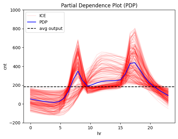
Explain it with global effect plots
# Initialize the Partial Dependence Plot (PDP) object
pdp = effector.PDP(
    X_test,  # Use the test set as background data
    predict,  # Prediction function
    feature_names=bike_sharing.feature_names,  # (optional) Feature names
    target_name=bike_sharing.target_name  # (optional) Target variable name
)

# Plot the effect of a feature
pdp.plot(
    feature=3,  # Select the 3rd feature (feature: hour)
    nof_ice=200,  # (optional) Number of Individual Conditional Expectation (ICE) curves to plot
    scale_x={"mean": bike_sharing.x_test_mu[3], "std": bike_sharing.x_test_std[3]},  # (optional) Scale x-axis
    scale_y={"mean": bike_sharing.y_test_mu, "std": bike_sharing.y_test_std},  # (optional) Scale y-axis
    centering=True,  # (optional) Center PDP and ICE curves
    show_avg_output=True,  # (optional) Display the average prediction
    y_limits=[-200, 1000]  # (optional) Set y-axis limits
)
Explain it with regional effect plots
# Initialize the Regional Partial Dependence Plot (RegionalPDP)
r_pdp = effector.RegionalPDP(
    X_test,  # Test set data
    predict,  # Prediction function
    feature_names=bike_sharing.feature_names,  # Feature names
    target_name=bike_sharing.target_name  # Target variable name
)

# Summarize the subregions of the 3rd feature (temperature)
r_pdp.summary(
    features=3,  # Select the 3rd feature for the summary
    scale_x_list=[  # scale each feature with mean and std
        {"mean": bike_sharing.x_test_mu[i], "std": bike_sharing.x_test_std[i]}
        for i in range(X_test.shape[1])
    ]
)
Feature 3 - Full partition tree:
🌳 Full Tree Structure:
───────────────────────
hr 🔹 [id: 0 | heter: 0.43 | inst: 3476 | w: 1.00]
    workingday = 0.00 🔹 [id: 1 | heter: 0.36 | inst: 1129 | w: 0.32]
        temp ≤ 6.50 🔹 [id: 3 | heter: 0.17 | inst: 568 | w: 0.16]
        temp > 6.50 🔹 [id: 4 | heter: 0.21 | inst: 561 | w: 0.16]
    workingday ≠ 0.00 🔹 [id: 2 | heter: 0.28 | inst: 2347 | w: 0.68]
        temp ≤ 6.50 🔹 [id: 5 | heter: 0.19 | inst: 953 | w: 0.27]
        temp > 6.50 🔹 [id: 6 | heter: 0.20 | inst: 1394 | w: 0.40]
--------------------------------------------------
Feature 3 - Statistics per tree level:
🌳 Tree Summary:
─────────────────
Level 0🔹heter: 0.43
    Level 1🔹heter: 0.31 | 🔻0.12 (28.15%)
        Level 2🔹heter: 0.19 | 🔻0.11 (37.10%)
The summary of feature hr (hour) says that its effect on the output is highly dependent on the value of features:
workingday, wheteher it is a workingday or nottemp, what is the temperature the specific hour
Let's see how the effect changes on these subregions!
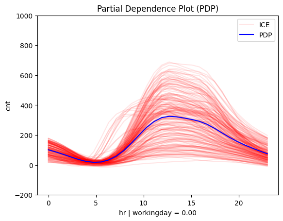
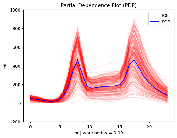
Is it workingday or not?
# Plot regional effects after the first-level split (workingday vs non-workingday)
for node_idx in [1, 2]:  # Iterate over the nodes of the first-level split
    r_pdp.plot(
        feature=3,  # Feature 3 (temperature)
        node_idx=node_idx,  # Node index (1: workingday, 2: non-workingday)
        nof_ice=200,  # Number of ICE curves
        scale_x_list=[  # Scale features by mean and std
            {"mean": bike_sharing.x_test_mu[i], "std": bike_sharing.x_test_std[i]}
            for i in range(X_test.shape[1])
        ],
        scale_y={"mean": bike_sharing.y_test_mu, "std": bike_sharing.y_test_std},  # Scale the target
        y_limits=[-200, 1000]  # Set y-axis limits
    )
 |
 |
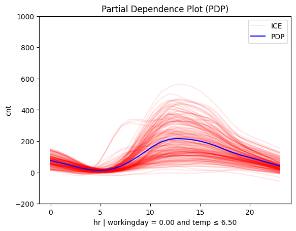
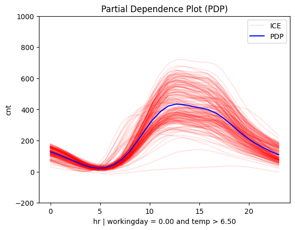
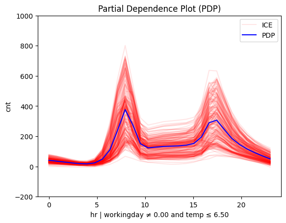
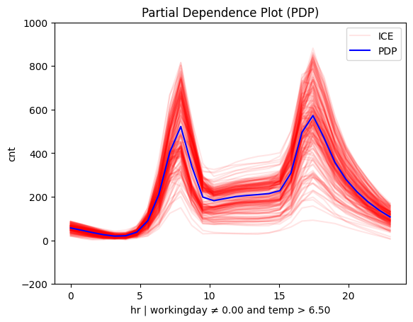
Is it hot or cold?
# Plot regional effects after second-level splits (workingday vs non-workingday and hot vs cold temperature)
for node_idx in [3, 4, 5, 6]:  # Iterate over the nodes of the second-level splits
    r_pdp.plot(
        feature=3,  # Feature 3 (temperature)
        node_idx=node_idx,  # Node index (hot/cold temperature and workingday/non-workingday)
        nof_ice=200,  # Number of ICE curves
        scale_x_list=[  # Scale features by mean and std
            {"mean": bike_sharing.x_test_mu[i], "std": bike_sharing.x_test_std[i]}
            for i in range(X_test.shape[1])
        ],
        scale_y={"mean": bike_sharing.y_test_mu, "std": bike_sharing.y_test_std},  # Scale target
        y_limits=[-200, 1000]  # Set y-axis limits
    )
 |
 |
 |
 |
Supported Methods
effector implements global and regional effect methods:
| Method | Global Effect | Regional Effect | Reference | ML model | Speed |
|---|---|---|---|---|---|
| PDP | PDP |
RegionalPDP |
PDP | any | Fast for a small dataset |
| d-PDP | DerPDP |
RegionalDerPDP |
d-PDP | differentiable | Fast for a small dataset |
| ALE | ALE |
RegionalALE |
ALE | any | Fast |
| RHALE | RHALE |
RegionalRHALE |
RHALE | differentiable | Very fast |
| SHAP-DP | ShapDP |
RegionalShapDP |
SHAP | any | Fast for a small dataset and a light ML model |
Method Selection Guide
From the runtime persepective there are three criterias:
- is the dataset
small(N<10K) orlarge(N>10K instances) ? - is the ML model
light(runtime < 0.1s) orheavy(runtime > 0.1s) ? - is the ML model
differentiableornon-differentiable?
Trust us and follow this guide:
light+small+differentiable=any([PDP, RHALE, ShapDP, ALE, DerPDP])light+small+non-differentiable:[PDP, ALE, ShapDP]heavy+small+differentiable=any([PDP, RHALE, ALE, DerPDP])heavy+small+non differentiable=any([PDP, ALE])big+not differentiable=ALEbig+differentiable=RHALE
Citation
If you use effector, please cite it:
@misc{gkolemis2024effector,
  title={effector: A Python package for regional explanations},
  author={Vasilis Gkolemis et al.},
  year={2024},
  eprint={2404.02629},
  archivePrefix={arXiv},
  primaryClass={cs.LG}
}
References
- Friedman, Jerome H. "Greedy function approximation: a gradient boosting machine." Annals of statistics (2001): 1189-1232.
- Apley, Daniel W. "Visualizing the effects of predictor variables in black box supervised learning models." arXiv preprint arXiv:1612.08468 (2016).
- Gkolemis, Vasilis, "RHALE: Robust and Heterogeneity-Aware Accumulated Local Effects"
- Gkolemis, Vasilis, "DALE: Decomposing Global Feature Effects Based on Feature Interactions"
- Lundberg, Scott M., and Su-In Lee. "A unified approach to interpreting model predictions." Advances in neural information processing systems. 2017.
- REPID: Regional Effect Plots with implicit Interaction Detection
- Decomposing Global Feature Effects Based on Feature Interactions
- Regionally Additive Models: Explainable-by-design models minimizing feature interactions
License
effector is released under the MIT License.


