rportion - data structure and operations for rectilinear polygons

The rportion library provides data structure to represent 2D rectilinear polygons (unions of 2D-intervals) in Python 3.9+. It is built upon the library portion and follows its concepts. The following features are provided:

• 2D-Intervals (rectangles) which can be open/closed and finite/infinite at every boundary
• intersection, union, complement and difference of rectilinear polygons
• iterator over all maximum rectangles inside and outside a given polygon

In the case of integers/floats it can be used to keep track of the area resulting from the union/difference of rectangles:

Internally the library uses an interval tree to represent a polygon.

Table of contents

• Installation
• Documentation & usage
  • Polygon creation
  • Polygon bounds & attributes
  • Polygon operations
  • Rectangle partitioning iterator
  • Maximum rectangle iterator
  • Boundary
  • Internal data structure
• Changelog
• Contributions
• License

Installation

rportion can be installed from PyPi with pip using

pip install rportion

Alternatively, clone the repository and run

pip install -e ".[test]"
python -m unittest discover -s tests

Note that `python

Documentation & usage

Polygon creation

Atomic polygons (rectangles) can be created by one of the following:

>>> import rportion as rp
>>> rp.ropen(0, 2, 0, 1)
(x=(0,2), y=(0,1))
>>> rp.rclosed(0, 2, 0, 1)
(x=[0,2], y=[0,1])
>>> rp.ropenclosed(0, 2, 0, 1)
(x=(0,2], y=(0,1])
>>> rp.rclosedopen(0, 2, 0, 1)
(x=[0,2), y=[0,1))
>>> rp.rsingleton(0, 1)
(x=[0], y=[1])
>>> rp.rempty()
(x=(), y=())

Polygons can also be created by using two intervals of the underlying library portion:

>>> import portion as P
>>> import rportion as rp
>>> rp.RPolygon.from_interval_product(P.openclosed(0, 2), P.closedopen(0, 1))
(x=(0,2], y=[0,1))

↑ back to top

Polygon bounds & attributes

An RPolygon defines the following properties

• empty is true if the polygon is empty.

  >>> rp.rclosed(0, 2, 1, 2).empty
  False
  >>> rp.rempty().empty
  True
  

• atomic is true if the polygon can be expressed by a single rectangle.

  >>> rp.rempty().atomic
  True
  >>> rp.rclosedopen(0, 2, 1, 2).atomic
  True
  >>> (rp.rclosed(0, 2, 1, 2) | rp.rclosed(0, 2, 1, 3)).atomic
  True
  >>> (rp.rclosed(0, 2, 1, 2) | rp.rclosed(1, 2, 1, 3)).atomic
  False
  

• enclosure is the smallest rectangle containing the polygon.

  >>> (rp.rclosed(0, 2, 0, 2) | rp.rclosed(1, 3, 0, 1)).enclosure
  (x=[0,3], y=[0,2])
  >>> (rp.rclosed(0, 1, -3, 3) | rp.rclosed(-P.inf, P.inf, -1, 1)).enclosure
  (x=(-inf,+inf), y=[-3,3])
  

• enclosure_x_interval is the smallest rectangle containing the polygon's extension in x-dimension.

  >>> (rp.rclosed(0, 2, 0, 2) | rp.rclosed(1, 3, 0, 1)).x_enclosure_interval
  x=[0,3]
  >>> (rp.rclosed(0, 1, -3, 3) | rp.rclosed(-P.inf, P.inf, -1, 1)).x_enclosure_interval
  (-inf,+inf)
  

• enclosure_y_interval is the smallest interval containing the polygon's extension in y-dimension.

  >>> (rp.rclosed(0, 2, 0, 2) | rp.rclosed(1, 3, 0, 1)).y_enclosure_interval
  [0,2]
  >>> (rp.rclosed(0, 1, -3, 3) | rp.rclosed(-P.inf, P.inf, -1, 1)).y_enclosure_interval
  [-3,3]
  

• x_lower, x_upper, y_lower and y_upper yield the boundaries of the rectangle enclosing the polygon.

  >>> p = rp.rclosedopen(0, 2, 1, 3)
  >>> p.x_lower, p.x_upper, p.y_lower, p.y_upper
  (0, 2, 1, 3)
  

• x_left, x_right, y_left and y_right yield the type of the boundaries of the rectangle enclosing the polygon.

  >>> p = rp.rclosedopen(0, 2, 1, 3)
  >>> p.x_left, p.x_right, p.y_left, p.y_right
  (CLOSED, OPEN, CLOSED, OPEN)
  

↑ back to top

Polygon operations

RPolygon instances support the following operations:

• p.intersection(other) and p & other return the intersection of two rectilinear polygons.

  >>> rp.rclosed(0, 2, 0, 2) & rp.rclosed(1, 3, 0, 1)
  (x=[1,2], y=[0,1])
  

• p.union(other) and p | other return the union of two rectilinear polygons.

  >>> rp.rclosed(0, 2, 0, 2) | rp.rclosed(1, 3, 0, 1)
  (x=[0,3], y=[0,1]) | (x=[0,2], y=[0,2])
  

  Note that the resulting polygon is represented by the union of all maximal rectangles contained in in the polygon, see Maximum rectangle iterators.
• p.complement() and ~p return the complement of the rectilinear polygon.

  >>> ~rp.ropen(-P.inf, 0, -P.inf, P.inf)
  ((x=[0,+inf), y=(-inf,+inf))
  

• p.difference(other) and p - other return the difference of two rectilinear polygons.

  rp.rclosed(0, 3, 0, 2) - rp.ropen(2, 4, 1, 3)
  (x=[0,3], y=[0,1]) | (x=[0,2], y=[0,2])
  

  Note that the resulting polygon is represented by the union of all maximal rectangles contained in in the polygon, see Maximum rectangle iterators.

↑ back to top

Rectangle partitioning iterator

The method rectangle_partitioning of a RPolygon instance returns an iterator over rectangles contained in the rectilinear polygon which disjunctively cover it. I.e.

>>> poly = rp.rclosedopen(2, 5, 1, 4) | rp.rclosedopen(1, 8, 2, 3) | rp.rclosedopen(6, 8, 1, 3)
>>> poly = poly - rp.rclosedopen(4, 7, 2, 4)
>>> list(poly.rectangle_partitioning())
[(x=[1,4), y=[2,3)), (x=[2,5), y=[1,2)), (x=[6,8), y=[1,2)), (x=[2,4), y=[3,4)), (x=[7,8), y=[2,3))]

which can be visualized as follows:

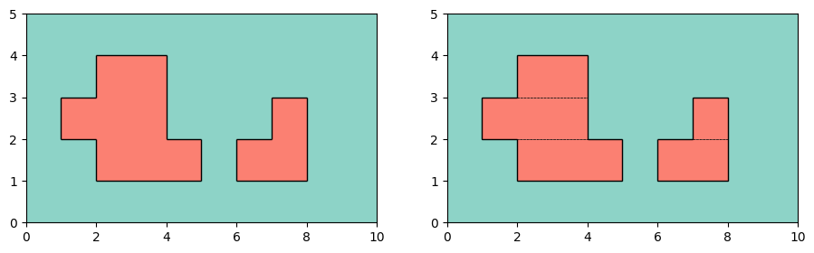
Left: Simple Rectilinear polygon. The red areas are part of the polygon.
Right: Rectangles in the portion are shown with black borderlines. As it is visible rectangle_partitioning prefers rectangles with long x-interval over rectangles with long y-interval.

↑ back to top

Maximum rectangle iterator

The method maximal_rectangles of a RPolygon instance returns an iterator over all maximal rectangles contained in the rectilinear polygon.

A maximal rectangle is rectangle in the polygon which is not a real subset of any other rectangle contained in the rectilinear polygon. I.e.

>>> poly = rp.rclosedopen(2, 5, 1, 4) | rp.rclosedopen(1, 8, 2, 3) | rp.rclosedopen(6, 8, 1, 3)
>>> poly = poly - rp.rclosedopen(4, 7, 2, 4)
>>> list(poly.maximal_rectangles())
[(x=[1, 4), y = [2, 3)), (x=[2, 5), y = [1, 2)), (x=[6, 8), y = [1, 2)), (x=[2, 4), y = [1, 4)), (x=[7, 8), y = [1, 3))]

which can be visualized as follows:

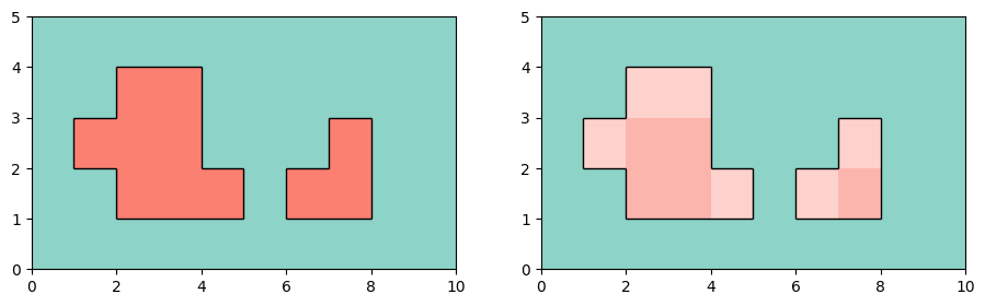
Left: Simple Rectilinear polygon. The red areas are part of the polygon.
Right: Maximal contained rectangles are drawn above each other transparently.

↑ back to top

Boundary

The method boundary of a RPolygon instance returns another RPolygon instance representing the boundary of the polygon. I.e.

>>> poly = rp.closed(0, 1, 2, 3)
>>> poly.boundary()
(x=[1,2], y=[3]) | (x=[1,2], y=[4]) | (x=[1], y=[3,4]) | (x=[2], y=[3,4])

↑ back to top

Internal data structure

The polygon is internally stored using an interval tree. Every node of the tree corresponds to an interval in x-dimension which is representable by boundaries (in x-dimension) present in the polygon. Each node contains an 1D-interval (by using the library portion) in y-dimension. Combining those 1D-intervals yields a rectangle contained in the polygon.

I.e. for the rectangle (x=[0, 2), y=[1, 3)) this can be visualized as follows.

  interval tree with      x-interval corresponding       y-interval stored in
 a lattice-like shape             to each node                each node
       ┌─x─┐                      ┌─(-∞,+∞)─┐                  ┌─()──┐
       │   │                      │         │                  │     │
     ┌─x─┬─x─┐               ┌─(-∞,2)──┬──[0,+∞)─┐          ┌─()──┬──()─┐
     │   │   │               │         │         │          │     │     │
     x   x   x            (-∞,0]     [0,2)     [2,+∞)      ()   [1,3)   ()

The class RPolygon used this model by holding three data structures.

• _x_boundaries: Sorted list of necessary boundaries in x-dimension with type (OPEN or CLOSED)
• _used_y_ranges: List of lists in a triangular shape representing the interval tree for the space occupied by the rectilinear polygon.
• _free_y_ranges: List of list in a triangular shape representing the interval tree of for the space not occupied by the rectilinear polygon.

Note that a separate data structure for the area outside the polygon is kept. This is done in order to be able to obtain the complement of a polygon efficiently.

For the example shown above this is:

>>> poly = rp.rclosedopen(0, 2, 1, 3)
>>> poly._x_boundaries
SortedList([(-inf, OPEN), (0, OPEN), (2, OPEN), (+inf, OPEN)])
>>> poly._used_y_ranges
[[(), (), ()], 
 [(), [1,3)], 
 [()]]
>>> poly._free_y_ranges
[[(-inf,1) | [3,+inf), (-inf,1) | [3,+inf), (-inf,+inf)], 
 [(-inf,1) | [3,+inf), (-inf,1) | [3,+inf)], 
 [(-inf,+inf)]]

You can use the function data_tree_to_string as noted below to print the internal data structure in a tabular format:

>>> poly = rp.rclosedopen(0, 2, 1, 3)
>>> print(data_tree_to_string(poly._x_boundaries, poly._used_y_ranges, 6))
                |  +inf     2     0
----------------+------------------
     -inf (OPEN)|    ()    ()    ()
      0 (CLOSED)|    () [1,3)
      2 (CLOSED)|    ()

>>> poly = rp.rclosedopen(2, 5, 1, 4) | rp.rclosedopen(1, 8, 2, 3) | rp.rclosedopen(6, 8, 1, 3)
>>> poly = poly - rp.rclosedopen(4, 7, 2, 4)
>>> print(data_tree_to_string(poly._x_boundaries, poly._used_y_ranges, 6))
                |  +inf     8     7     6     5     4     2     1
----------------+------------------------------------------------
     -inf (OPEN)|    ()    ()    ()    ()    ()    ()    ()    ()
      1 (CLOSED)|    ()    ()    ()    ()    () [2,3) [2,3)
      2 (CLOSED)|    ()    ()    ()    () [1,2) [1,4)
      4 (CLOSED)|    ()    ()    ()    () [1,2)
      5 (CLOSED)|    ()    ()    ()    ()
      6 (CLOSED)|    () [1,2) [1,2)
      7 (CLOSED)|    () [1,3)

def data_tree_to_string(x_boundaries,
                        y_intervals,
                        spacing: int):
    col_space = 10
    n = len(y_intervals)
    msg = " " * (spacing + col_space) + "|"
    for x_b in x_boundaries[-1:0:-1]:
        msg += f"{str(x_b.val):>{spacing}}"
    msg += "\n" + f"-" * (spacing+col_space) + "+"
    for i in range(n):
        msg += f"-" * spacing
    msg += "\n"
    for i, row in enumerate(y_intervals):
        x_b = x_boundaries[i]
        msg += f"{str((~x_b).val) + ' (' + str((~x_b).btype) + ')':>{spacing+ col_space}}|"
        for val in row:
            msg += f"{str(val):>{spacing}}"
        msg += "\n"
    return msg

↑ back to top

Changelog

This library adheres to a semantic versioning scheme. See CHANGELOG.md for the list of changes.

Contributions

Contributions are very welcome! Feel free to report bugs or suggest new features using GitHub issues and/or pull requests.

License

Distributed under MIT License.