PlanetaRY spanGLES: general photometry of planets, rings and shadows

Project description
Pryngles
PlanetaRY spaNGLES


Pryngles is a Python package intended to produce useful
visualizations of the geometric configuration of a ringed exoplanet
(an exoplanet with a ring or exoring for short) and more importantly
to calculate the light curve produced by this kind of planets. The
model behind the package has been developed in an effort to predict
the signatures that exorings may produce not only in the light curve
of transiting exoplanets (a problem that has been extensively studied)
but also in the light of stars having non-transiting exoplanets (the
bright side of the light curve).
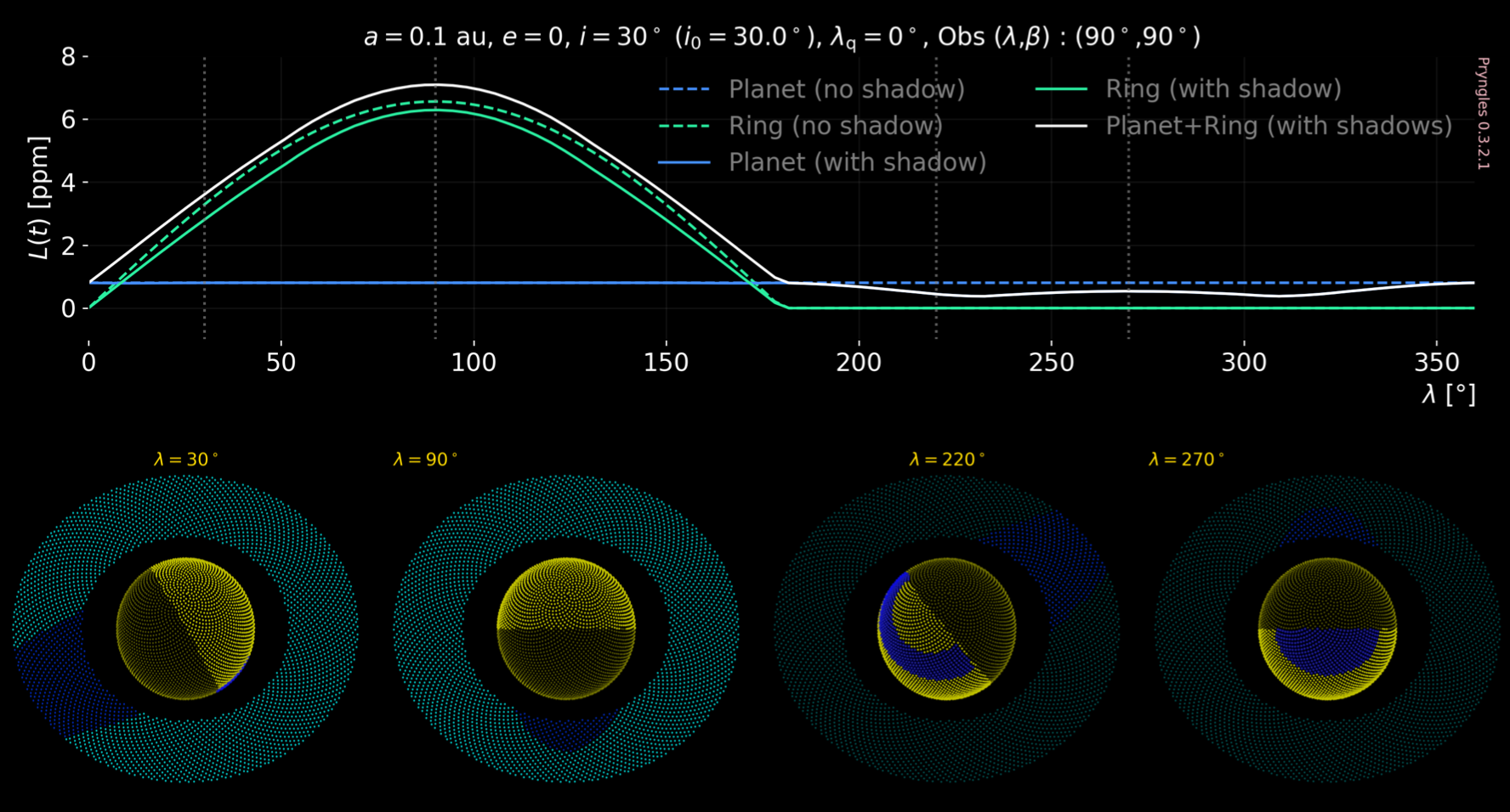
This is an example of what can be done with Pryngles:
For the science behind the model please refer to the following papers:
Zuluaga, J.I., Sucerquia, M. & Alvarado-Montes, J.A. (2022), The bright side of the light curve: a general photometric model for non-transiting exorings, Astronomy and Computing 40 (2022) 100623, arXiv:2207.08636.
Sucerquia, M., Alvarado-Montes, J. A., Zuluaga, J. I., Montesinos, M., & Bayo, A. (2020), Scattered light may reveal the existence of ringed exoplanets. Monthly Notices of the Royal Astronomical Society: Letters, 496(1), L85-L90.
Download and install
pryngles is available in PyPI, https://pypi.org/project/pryngles/.
To install it, just execute:
pip install -U pryngles
If you prefer, you may download and install from the sources.
Quick start
Import the package and some useful utilities:
import pryngles as pr
from pryngles import Consts
NOTE: If you are working in
Google Colabbefore producing any plot please load the matplotlib backend:
%matplotlib inline
Any calculation in Pryngles starts by creating a planetary system:
sys=pr.System()
S=sys.add(kind="Star",radius=Consts.rsun/sys.ul,limb_coeffs=[0.65])
P=sys.add(kind="Planet",parent=S,a=0.2,e=0.0,radius=Consts.rsaturn/sys.ul)
R=sys.add(kind="Ring",parent=P,fi=1.5,fe=2.5,i=30*Consts.deg)
RP=sys.ensamble_system(lamb=90*Consts.deg,beta=90*Consts.deg)
In the example before the planet has a ring extending from 1.5 to 2.5 planetary radius which is inclined 30 degrees with respect to the orbital plane. It has an orbit with semimajor axis of 0.2 and eccentricity 0.0.
Once the system is set we can ensamble a simulation, ie. creating an object able to produce a light-curve.
RP=sys.ensamble_system()
To see how the surface of the planet and the rings looks like run:
RP.plotRingedPlanet()
You may change the position of the star in the orbit and see how the appearance of the planet changes:
RP.changeStellarPosition(45*Consts.deg)
RP.plotRingedPlanet()
Below is the sequence of commands to produce your first light curve:
import numpy as np
RP.changeObserver([90*Consts.deg,30*Consts.deg])
lambs=np.linspace(+0.0*Consts.deg,+360*Consts.deg,100)
Rps=[]
Rrs=[]
ts=[]
for lamb in lambs:
    RP.changeStellarPosition(lamb)
    ts+=[RP.t*sys.ut/Consts.day]
    RP.updateOpticalFactors()
    RP.updateDiffuseReflection()
    Rps+=[RP.Rip.sum()]
    Rrs+=[RP.Rir.sum()]

ts=np.array(ts)
Rps=np.array(Rps)
Rrs=np.array(Rrs)

#Plot
import matplotlib.pyplot as plt
fig=plt.figure()
ax=fig.gca()
ax.plot(ts,Consts.ppm*Rps,label="Planet")
ax.plot(ts,Consts.ppm*Rrs,label="Ring")
ax.plot(ts,Consts.ppm*(Rps+Rrs),label="Planet+Ring")

ax.set_xlabel("Time [days]")
ax.set_ylabel("Flux anomaly [ppm]")
ax.legend();
And voilà!
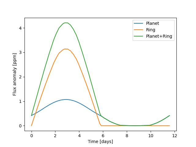
Let's have some Pryngles.
Realistic scattering and polarization
Starting in version 0.9.x, Pryngles is able to compute fluxes using a more realistic model for scattering that includes polarization. The new features are not yet flexible enough but they can be used to create more realistic light curves.
These new features are based on the science and Fortran code developed
by Prof. Daphne Stam and collaborators, and adapted to Pryngles
environment by Allard Veenstra (Fortran and Python wrapping) and Jorge
I. Zuluaga (translation to C and ctypes). For the science behind the
scattering and polarization code see:
Rossi, L., Berzosa-Molina, J., & Stam, D. M. (2018). PyMieDAP: a Python–Fortran tool for computing fluxes and polarization signals of (exo) planets. Astronomy & Astrophysics, 616, A147. arXiv:1804.08357
Below is a simple example of how to compute the light curve of a ringed planet whose atmosphere and ring scatters reallistically the light of the star. The code compute the components of the Stokes vector and the degree of polarization of the diffusely reflected light on the system.
As shown in the example before, we first need to create the system:
nspangles=1000
sys = pr.System()
S=sys.add(kind="Star",radius=Consts.rsun/sys.ul,limb_coeffs=[0.65])
P=sys.add(kind="Planet",primary=S,a=3,e=0.0,
          radius=Consts.rsaturn/sys.ul,nspangles=nspangles)
R=sys.add(kind="Ring",primary=P,fi=1.5,fe=2.25,
          i=30*Consts.deg,roll=90*Consts.deg,nspangles=nspangles)
RP=sys.ensamble_system()
Then generate the light curve:
import numpy as np
from tqdm import tqdm
RP.changeObserver([-90*Consts.deg,60*Consts.deg])
lambs=np.linspace(90*Consts.deg,450*Consts.deg,181)

ts=[]
Rps=[]
Rrs=[]
Pp = []
Pr = []
Ptot=[]
for lamb in tqdm(lambs):
    RP.changeStellarPosition(lamb)
    ts+=[RP.t*RP.CU.UT]
    RP.updateOpticalFactors()
    RP.updateReflection()
    Rps+=[RP.Rip.sum()]
    Rrs+=[RP.Rir.sum()]
    Pp += [RP.Ptotp]
    Pr += [RP.Ptotr]
    Ptot+=[RP.Ptot]

ts=np.array(ts)
Rps=np.array(Rps)
Rrs=np.array(Rrs)
Pp=np.array(Pp)
Pr=np.array(Pr)
Ptot=np.array(Ptot)
And plot it:
#Plot
fig,axs=plt.subplots(2,1,figsize=(6,6),sharex=True)

ax=axs[0]
ax.plot(lambs*180/np.pi-90,Rps,label="Planet")
ax.plot(lambs*180/np.pi-90,Rrs,label="Ring")
ax.plot(lambs*180/np.pi-90,Rps+Rrs,label="Planet + Ring")
ax.set_ylabel("Flux anomaly [ppm]")
ax.legend()
ax.grid()
pr.Plot.pryngles_mark(ax)

ax=axs[1]
ax.plot(lambs*180/np.pi-90,Pp,label="Planet")
ax.plot(lambs*180/np.pi-90,Pr,label="Ring")
ax.plot(lambs*180/np.pi-90,Ptot,label="Planet + Ring")
ax.set_ylabel("Degree of polarization [-]")
ax.legend()
ax.grid()
pr.Plot.pryngles_mark(ax)

ax=axs[1]
ax.set_xlabel("True anomaly [deg]")
fig.tight_layout()
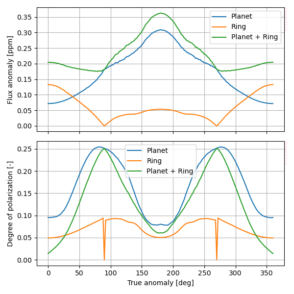
The resulting polarization and light-curve will be:
Tutorials
We have prepared several Jupyter tutorials to guide you in the usage
of the package. The tutorials evolve as the package is being optimized.
-
Quickstart [Download, Google Colab]. In this tutorial you will learn the very basics about the package.
-
Developers [Download, Google Colab]. In this tutorial you will find a detailed description and exemplification of almost every part of the package. It is especially intended for developers, however it may also be very useful for finding code snippets useful for science applications. As expected, it is under construction as the package is being developed.
Examples
Working with Pryngles we have created several Jupyter notebooks to
illustrate many of its capabilities. In the examples below you will
find the package at work to do actual science:
- Full-science exploration [Download, Google Colab]. In this example we include the code we used to generate the plots of the release paper arXiv:2207.08636 as a complete example of how the package can be used in a research context.
Disclaimer
This is the disco version of Pryngles. We are improving resolution, performance, modularity and programming standards for future releases.
What's new
For a detailed list of the newest features introduced in the latest releases pleas check What's new.
This package has been designed and written originally by Jorge I. Zuluaga, Mario Sucerquia & Jaime A. Alvarado-Montes with the contribution of Allard Veenstra (C) 2022
Release history Release notifications | RSS feed


Download files
Download the file for your platform. If you're not sure which to choose, learn more about installing packages.
Source Distribution
Built Distribution
Hashes for pryngles-0.9.10-cp39-cp39-macosx_10_9_x86_64.whl
| Algorithm | Hash digest | |
|---|---|---|
| SHA256 | 26397c84a53a0805beb2a9d12d853d055d77d6493fdb309f4d1a3d3c1e6cebda |
|
| MD5 | 91c05f259665a75285fb4e5a32b72a11 |
|
| BLAKE2b-256 | ba0bb323a6e6952658edf55c0f6b3a6732bc948e6df0b7bd76334dcada9162e9 |


