Python package to build and manipulate temporal NetworkX graphs.

Project description
networkx-temporal
Python package to build and manipulate temporal NetworkX graphs.
Requirements
- Python>=3.7
- networkx>=2.1
- pandas>=1.1.0
Install
Package is available to install on PyPI:
pip install networkx-temporal
Usage
The code provided as example below is also available as an interactive Jupyter notebook (open on Colab).
- Build temporal graph: basics on manipulating a
networkx-temporalgraph object; - Common metrics: common metrics available from
networkx; - Convert from static to temporal graph: converting
networkxgraphs tonetworkx-temporal; - Transform temporal graph: converting
networkx-temporalto other graph formats or representations; - Detect temporal communities: example of temporal community detection with a
networkx-temporalobject.
Build temporal graph
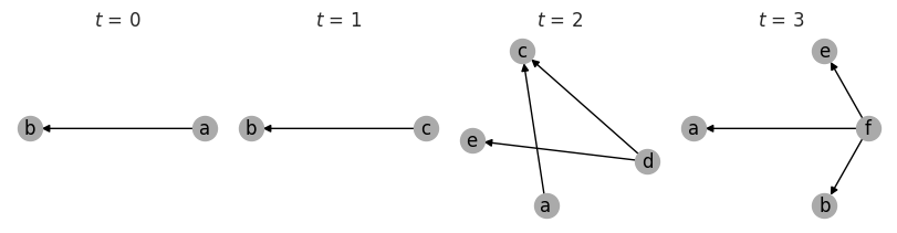
The Temporal{Di,Multi,MultiDi}Graph class uses NetworkX graphs internally to allow easy manipulation of its data structures:
import networkx_temporal as tx
from networkx_temporal.tests.example import draw_temporal_graph
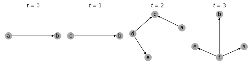
TG = tx.TemporalGraph(directed=True, multigraph=False, t=4)
TG[0].add_edge("a", "b")
TG[1].add_edge("c", "b")
TG[2].add_edge("d", "c")
TG[2].add_edge("d", "e")
TG[2].add_edge("a", "c")
TG[3].add_edge("f", "e")
TG[3].add_edge("f", "a")
TG[3].add_edge("f", "b")
draw_temporal_graph(TG, figsize=(8, 2))
Slice into temporal bins
Once initialized, a specified number of bins can be returned in a new object of the same type using slice:
TGS = TG.slice(bins=2)
draw_temporal_graph(TGS, figsize=(4, 2))
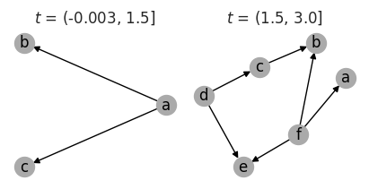
By default, created bins are composed of non-overlapping edges and might have uneven size. To balance them, pass qcut=True:
TGS = TG.slice(bins=2, qcut=True)
draw_temporal_graph(TGS, figsize=(4, 2))
Note that in some cases, qcut may not be able to split the graph into the number of bins requested and will instead return the maximum number of bins possible. Other exceptions can be worked around by setting duplicates=True to allow duplicate edges in bins, or rank_first=True to balance snapshots considering the order in which nodes or edges appear.
Convert to directed or undirected
We can easily convert the edge directions by calling the same methods available from networkx:
TG.to_undirected()
TG.to_directed()
Common metrics
All methods implemented by networkx, e.g., degree, are also available to be executed sequentially on the stored time slices.
A few additional methods that consider all time slices are also implemented for convenience, e.g., temporal_degree and temporal_neighbors.
Degree centrality
TG.degree()
# TG.in_degree()
# TG.out_degree()
TG.temporal_degree()
# TG.temporal_in_degree()
# TG.temporal_out_degree()
Or to obtain the degree of a specific node:
TG[0].degree("a")
# TG[0].in_degree("a")
# TG[0].out_degree("a")
TG.temporal_degree("a")
# TG.temporal_in_degree("a")
# TG.temporal_out_degree("a")
Node neighborhoods
TG.neighbors("c")
To obtain the temporal neighborhood of a node considering all time steps, use the method temporal_neighbors:
TG.temporal_neighbors("c")
Order and size
To get the number of nodes and edges in each time step:
print("Order:", TG.order())
print("Size:", TG.size())
Temporal order and size
The temporal order and size are respectively defined as the length of TG.temporal_nodes(), i.e., unique nodes in all time steps, and the length of TG.temporal_size(), i.e., sum of edges or interactions among nodes in all time steps.
print("Temporal nodes:", TG.temporal_order())
print("Temporal edges:", TG.temporal_size())
Total number of nodes and edges
To get the actual number of nodes and edges across all time steps:
print("Total nodes:", TG.total_nodes())  # TG.total_nodes() != TG.temporal_order()
print("Total edges:", TG.total_edges())  # TG.total_edges() == TG.temporal_size()
Convert from static to temporal graph
Static graphs can also carry temporal information either in the node- or edge-level attributes.
Slicing a graph into bins usually result in the same number of edges, but a higher number of nodes, as they may appear in more than one snapshot to preserve edge information.
In the example below, we create a static multigraph in which both nodes and edges are attributed with the time step t in which they are observed:
import networkx as nx

G = nx.MultiDiGraph()

G.add_nodes_from([
    ("a", {"t": 0}),
    ("b", {"t": 0}),
    ("c", {"t": 1}),
    ("d", {"t": 2}),
    ("e", {"t": 3}),
    ("f", {"t": 3}),
])

G.add_edges_from([
    ("a", "b", {"t": 0}),
    ("c", "b", {"t": 1}),
    ("d", "c", {"t": 2}),
    ("d", "e", {"t": 2}),
    ("a", "c", {"t": 2}),
    ("f", "e", {"t": 3}),
    ("f", "a", {"t": 3}),
    ("f", "b", {"t": 3}),
])
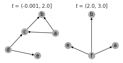
Node-level time attributes
Converting a static graph with node-level temporal data to a temporal graph object (node_level considers the source node's time by default when slicing edges):
TG = tx.from_static(G).slice(attr="t", attr_level="node", node_level="source", bins=None, qcut=None)
draw_temporal_graph(TG, figsize=(8, 2))
Note that considering node-level attributes resulted in placing the edge (a, c, 2) in $t=0$ instead, as the source node a attribute is set to t=0:
G.nodes(data=True)["a"]
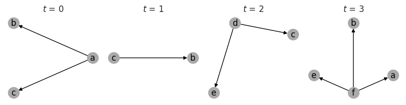
Edge-level time attributes
Converting a static graph with edge-level temporal data to a temporal graph object (edge's time applies to both source and target nodes):
TG = tx.from_static(G).slice(attr="t", attr_level="edge", bins=None, qcut=None)
draw_temporal_graph(TG, figsize=(8, 2))
In this case, considering edge-level attributes results in placing the edge (a, c, 2) in $t=2$, as expected.
Transform temporal graph
Once a temporal graph is instantiated, some methods are implemented that allow converting it or returning snaphots, events or unified temporal graphs.
to_static: returns a single graph with unique nodes, does not support dynamic node attributes;to_unified: returns a single graph with non-unique nodes, supports dynamic node attributes;to_snapshots: returns a list of graphs with possibly repeated nodes among snapshots;to_events: returns a list of edge-level events as 3-tuples or 4-tuples, without attributes.
Convert to different object type
Temporal graphs may be converted to a different object type by calling convert_to or passing to={package} to the above methods, provided package is locally installed. Supported formats:
| Package | Parameter | Alias |
|---|---|---|
| Deep Graph Library | dgl |
- |
| graph-tool | graph_tool |
gt |
| igraph | igraph |
ig |
| NetworKit | networkit |
nk |
| PyTorch Geometric | torch_geometric |
pyg |
tx.convert_to(G, "igraph")
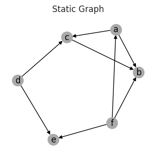
Static graph
Builds a static or flattened graph containing all the edges found at each time step:
G = TG.to_static()
draw_temporal_graph(G, suptitle="Static Graph")
Snapshot-based temporal graph
The snapshot-based temporal graph (STG) is a list of graphs directly accessible under data in the temporal graph object:
STG = TG.to_snapshots()
# STG == TG.data
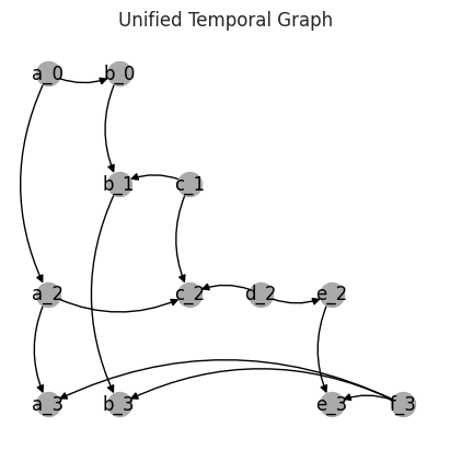
Unified temporal graph
The unified temporal graph (UTG) is a single graph that contains the original data plus proxy nodes and edge couplings connecting sequential temporal nodes.
UTG = TG.to_unified(add_couplings=True)
nodes = sorted(TG.temporal_nodes())
pos = {node: (nodes.index(node.rsplit("_")[0]), -int(node.rsplit("_")[1])) for node in UTG.nodes()}
draw_temporal_graph(UTG, pos=pos, figsize=(4, 4), connectionstyle="arc3,rad=0.25", suptitle="Unified Temporal Graph")
Event-based temporal graph
An event-based temporal graph (ETG) is a sequence of 3- or 4-tuple edge-based events.
-
3-tuples:
(u, v, t), where elements are the source node, target node, and time step of the observed event (also known as a stream graph); -
4-tuples:
(u, v, t, e), whereeis either a positive (1) or negative (-1) unity for edge addition and deletion, respectively.
ETG = TG.to_events()  # stream=True (default)
ETG

# [('a', 'b', 0),
#  ('c', 'b', 1),
#  ('a', 'c', 2),
#  ('d', 'c', 2),
#  ('d', 'e', 2),
#  ('f', 'e', 3),
#  ('f', 'a', 3),
#  ('f', 'b', 3)]
ETG = TG.to_events(stream=False)
ETG

# [('a', 'b', 0, 1),
#  ('c', 'b', 1, 1),
#  ('a', 'b', 1, -1),
#  ('a', 'c', 2, 1),
#  ('d', 'c', 2, 1),
#  ('d', 'e', 2, 1),
#  ('c', 'b', 2, -1),
#  ('f', 'e', 3, 1),
#  ('f', 'a', 3, 1),
#  ('f', 'b', 3, 1),
#  ('a', 'c', 3, -1),
#  ('d', 'c', 3, -1),
#  ('d', 'e', 3, -1)]
Convert back to TemporalGraph object
Functions to convert a newly created STG, ETG, or UTG back to a temporal graph object are also implemented.
tx.from_snapshots(STG)
tx.from_events(ETG, directed=False, multigraph=True)
tx.from_unified(UTG)
Detect temporal communities
The leidenalg package implements community detection algorithms on snapshot-based temporal graphs.
Depending on the objectives, temporal community detection may bring significant advantages on what comes to descriptive tasks and post-hoc network analysis.
Let's first use the Stochastic Block Model to construct a temporal graph of 4 snapshots, in which each of the five clusters of five nodes each continuously mix together:
snapshots = 4   # Temporal snapshots to creaete.
clusters = 5    # Number of clusters/communities.
order = 5       # Nodes in each cluster.
intra = .9      # High probability of intra-community edges.
inter = .1      # Low initial probability of inter-community edges.
change = .5    # Change in intra- and inter-community edges over time.

# Get probabilities for each snapshot.
probs = [[[(intra if i == j else inter) + (t * (change/snapshots) * (-1 if i == j else 1))
            for j in range(clusters)
        ] for i in range(clusters)
    ] for t in range(snapshots)]

# Create graphs from probabilities.
graphs = {}
for t in range(snapshots):
    graphs[t] = nx.stochastic_block_model(clusters*[order], probs[t], seed=10)
    graphs[t].name = t

# Create temporal graph from snapshots.
TG = tx.from_snapshots(graphs)
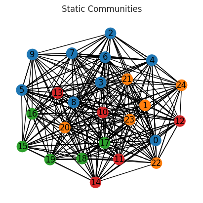
Static community detection
On the static graph (flattened)
Running the Leiden algorithm on the static graph to obtain the community modules fails to retrieve the five communities in the network:
import leidenalg as la

c = plt.cm.tab10.colors

membership = la.find_partition(
    TG.to_static("igraph"),
    la.ModularityVertexPartition,
    n_iterations=-1,
    seed=0,
)

node_color = [c[m] for m in membership.membership]

draw_temporal_graph(TG.to_static(), figsize=(4, 4), node_color=node_color, suptitle="Static Communities")
We can plot all four generated snapshots, while keeping the community assignments from the previous run:
draw_temporal_graph(TG, figsize=(12, 4), node_color=node_color, suptitle="Static Communities")
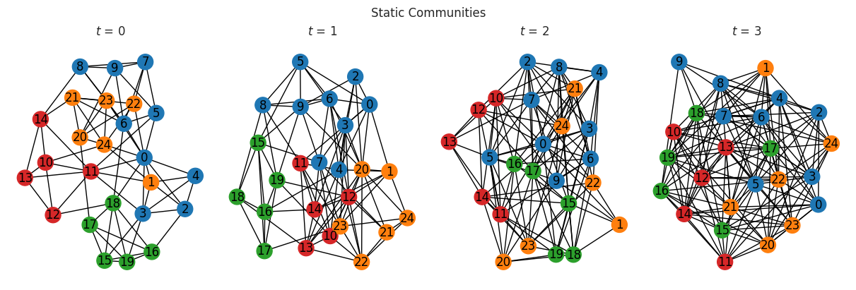
Note that running the same algorithm on the unified temporal graph also yields no significant advantages in terms of correctly retrieving the five clusters.
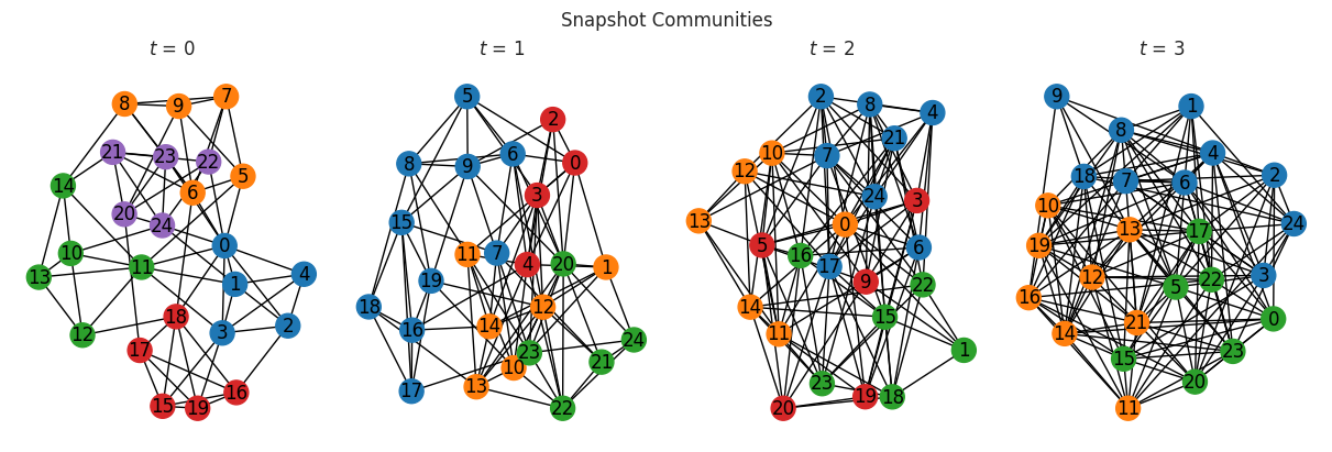
On the snapshots (individually)
Running the same algorithm on each of the generated snapshots instead retrieves the correct clusters on the first snapshot only.
Although results may seem initially better, we lose the community indices previously assigned to nodes in previous snapshots, represented by their different colors:
temporal_opts = {}

for t in range(len(TG)):
    membership = la.find_partition(
        TG[t:t+1].to_static("igraph"),
        la.ModularityVertexPartition,
        n_iterations=-1,
        seed=0,
    )
    temporal_opts[t] = {
        "node_color": [c[m] for m in membership.membership]
    }

draw_temporal_graph(TG, nrows=1, ncols=4, figsize=(12, 4), suptitle="Snapshot Communities", temporal_opts=temporal_opts)
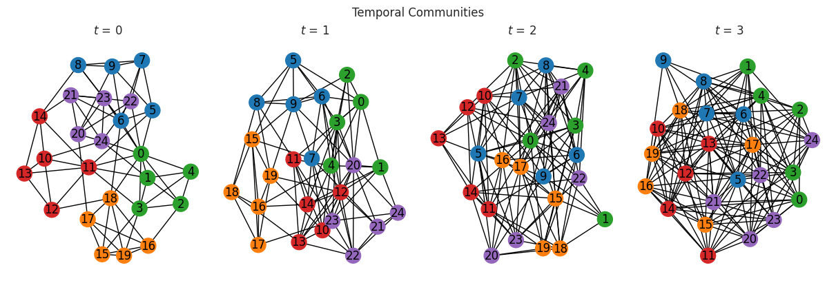
Temporal community detection
Detecting temporal communities instead allows us to correctly retrieve the clusters in all snapshots, while maintaining their indices/colors over time.
The interslice_weight among temporal nodes in a sequence of snapshots defaults to 1.0 in unweighted graphs and may be adjusted accordingly:
temporal_membership, improvement = la.find_partition_temporal(
    TG.to_snapshots("igraph"),
    la.ModularityVertexPartition,
    interslice_weight=1.0,
    n_iterations=-1,
    seed=0,
    vertex_id_attr="_nx_name"
)

temporal_opts = {
    t: {"node_color": [c[m] for m in temporal_membership[t]]}
    for t in range(len(TG))
}

draw_temporal_graph(TG, nrows=1, ncols=4, figsize=(12, 4), suptitle="Temporal Communities", temporal_opts=temporal_opts)
References
Release history Release notifications | RSS feed


Download files
Download the file for your platform. If you're not sure which to choose, learn more about installing packages.
Source Distribution
Built Distribution
Hashes for networkx_temporal-1.0b7-py3-none-any.whl
| Algorithm | Hash digest | |
|---|---|---|
| SHA256 | bd9a4287d1f2e15464ddf84b4cad0c39abe61eadade55fc3595072710f3c4185 |
|
| MD5 | 74a2d4820d16165cc9c1d6670630bd42 |
|
| BLAKE2b-256 | 5d46f7304e5a6468fc22cd9be1fd388980fbffa5a78cf0c9a4838d343dca3fe8 |


