LSNMS

Speeding up Non Maximum Suppression with a multiclass support ran on very large images by a several folds factor, using a sparse implementation of NMS. This project becomes useful in the case of very high dimensional images data, when the amount of predicted instances to prune becomes considerable (> 10,000 objects).

Installation

This project is fully installable with pip:

pip install lsnms --upgrade

or by cloning this repo with poetry

git clone https://github.com/remydubois/lsnms
cd lsnms/
poetry install

Only dependencies are numpy and numba.

Example usage:

import numpy as np
from lsnms import nms, wbc

# Create boxes: approx 30 pixels wide / high in Pascal VOC format:
# bbox = (x0, y0, x1, y1) with x1 > x0, y1 > y0
image_size = 10_000
n_predictions = 10_000
topleft = np.random.uniform(0.0, high=image_size, size=(n_predictions, 2))
wh = np.random.uniform(15, 45, size=topleft.shape)
boxes = np.concatenate([topleft, topleft + wh], axis=1).astype(np.float64)
# Create scores
scores = np.random.uniform(0., 1., size=(len(boxes), ))

# Create class_ids if multiclass, 3 classes here
class_ids = np.random.randint(0, 2, size=(len(boxes), ))

# Apply NMS
# During the process, overlapping boxes are queried using a R-Tree, ensuring a log-time search
keep = nms(boxes, scores, iou_threshold=0.5)
# Or, in a multiclass setting
keep = nms(boxes, scores, iou_threshold=0.5, class_ids=class_ids)
boxes = boxes[keep]
scores = scores[keep]

# Apply WBC
pooled_boxes, pooled_scores, cluster_indices = wbc(boxes, scores, iou_threshold=0.5)

Description

Non Maximum Suppression

A nice introduction of the non maximum suppression algorithm can be found here: https://www.coursera.org/lecture/convolutional-neural-networks/non-max-suppression-dvrjH. Basically, NMS discards redundant boxes in a set of predicted instances. It is an essential - and often unavoidable, step of object detection pipelines.

Scaling up the Non Maximum Suppression process

Complexity

• In the best case scenario, NMS is a linear-complex process (O(n)): if all boxes are perfectly overlapping, then one pass of the algorithm discards all the boxes except the highest scoring one.
• In worst case scenario, NMS is a quadratic-complex operation (one needs to perform n * (n - 1) / 2 iou comparisons): if all boxes are perfectly disconnected, each NMS step will discard only one box (the highest scoring one, by decreasing order of score). Hence, one needs to perform (n-1) + (n-2) + ... + 1 = n * (n - 1) / 2 iou computations.

Working with huge images

When working with high-dimensional images (such as satellital or histology images), one often runs object detection inference by patching (with overlap) the input image and applying NMS to independant patches. Because patches do overlap, a final NMS needs to be re-applied afterward. In that final case, one is close to be in the worst case scenario since each NMS step will discard only a very low amount of candidate instances (actually, pretty much the amount of overlapping passes over each instance, usually <= 10). Hence, depending on the size of the input image, computation time can reach several minutes on CPU. A more natural way to speed up NMS could be through parallelization, like it is done for GPU-based implementations, but:

1. Efficiently parallelizing NMS is not a straightforward process
2. If too many instances are predicted, GPU VRAM will often not be sufficient, retaining one from using GPU accelerators
3. The process remains quadratic, and does not scale well.

LSNMS

This project offers a way to overcome the aforementioned issues elegantly:

1. Before the NMS process, a R-Tree is built on bounding boxes (in a O(n*log(n)) time)
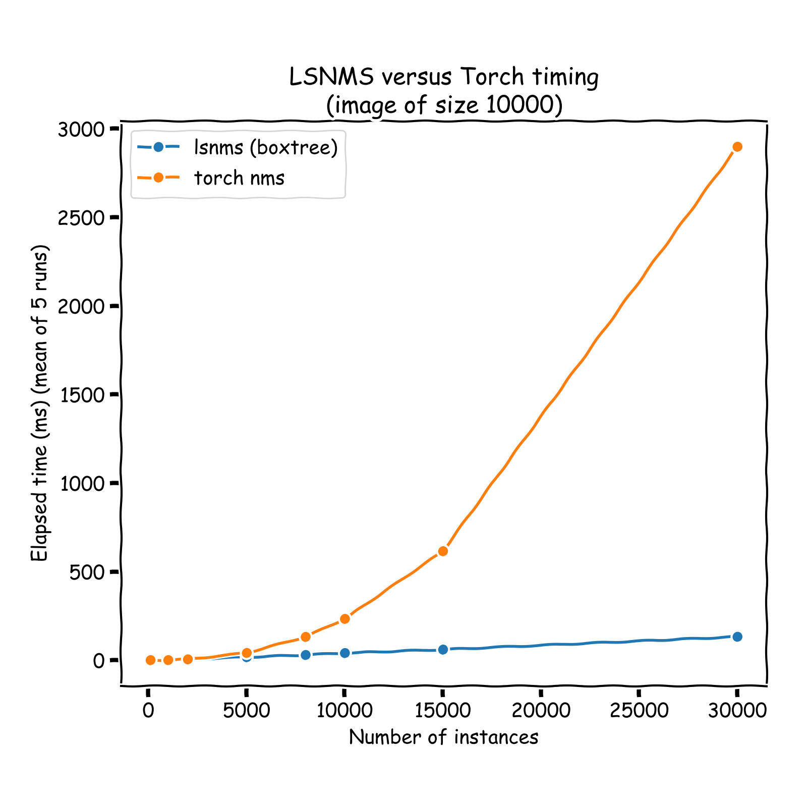
2. At each NMS step, only boxes overlapping with the current highest scoring box are queried in the tree (in a O(log(n)) complexity time), and only those neighbors are considered in the pruning process: IoU computation + pruning if necessary. Hence, the overall NMS process is turned from a O(n**2) into a O(n * log(n)) process. See a comparison of run times on the graph below (results obtained on sets of instances whose coordinates vary between 0 and 10,000 (x and y)). A nice introduction of R-Tree can be found here: https://iq.opengenus.org/r-tree/.

Note that the timing reported below are all inclusive: it notably includes the tree building process, otherwise comparison would not be fair.

For the sake of speed, this repo is entirely (including the binary tree) built using Numba's just-in-time compilation.

Concrete example: Some tests were ran considering ~ 40k x 40k pixels images, and detection inference ran on 512 x 512 overlapping patches (256-strided). Aproximately 300,000 bounding boxes (post patchwise NMS) resulted. Naive NMS ran in approximately 5 minutes on modern CPU, while this implementation ran in 5 seconds, hence offering a close to 60 folds speed up.

Going further: weighted box clustering

For the sake of completeness, this repo also implements a variant of the Weighted Box Clustering algorithm (from https://arxiv.org/pdf/1811.08661.pdf). Since NMS can artificially push up confidence scores (by selecting only the highest scoring box per instance), WBC overcomes this by averaging box coordinates and scores of all the overlapping boxes (instead of discarding all the non-maximally scored overlaping boxes).

Disclaimer:

1. The tree implementation could probably be further optimized, see implementation notes below.
2. Much simpler implementation could rely on existing KD-Tree implementations (such as sklearn's), query the tree before NMS, and tweak the NMS process to accept tree query's result. This repo implements it from scratch in full numba for the sake of completeness and elegance.
3. The main parameter deciding the speed up brought by this method is (along with the amount of instances) the density of boxes over the image: in other words, the amount of overlapping boxes trimmed at each step of the NMS process. The lower the density of boxes, the higher the speed up factor.
4. Due to numba's compiling process, the first call to each jitted function might lag a bit, second and further function calls (per python session) should not suffer this overhead.

-> Will I benefit from this sparse NMS implementation ? As said above, the main parameter guiding speed up from naive NMS is instance (or boxes) density (rather than image size or amount of instances):

• If a million boxes overlap perfectly on a 100k x 100k pixels image, no speed up will be obersved (even a slow down, related to tree building time)
• If 1,000 boxes are far appart from each other on a small image, the optimal speed up will be observed (with a good choice of neighborhood radius query)

Implementations notes

Tree implementation

Due to Numba compiler's limitations, tree implementations has some specificities: Because jit-class methods can not be recursive, the tree building process (node splitting + children instanciation) can not be entirely done inside the Node.__init__ method:

• Otherwise, the __init__ method would be recursive (children instanciation)
• However, methods can call recursive (instance-external) functions: a build function is dedicated to this
• Hence the tree building process must be as follows:

# instanciate root
root = Node(data, leaf_size=16)
# recursively split and attach children if necessary
root.build()  # This calls build(root) under the hood

• For convenience: a wrapper class RTree was implemented, encapsulating the above steps in __init__:

tree = RTree(data, leaf_size=16)

Multiclass support

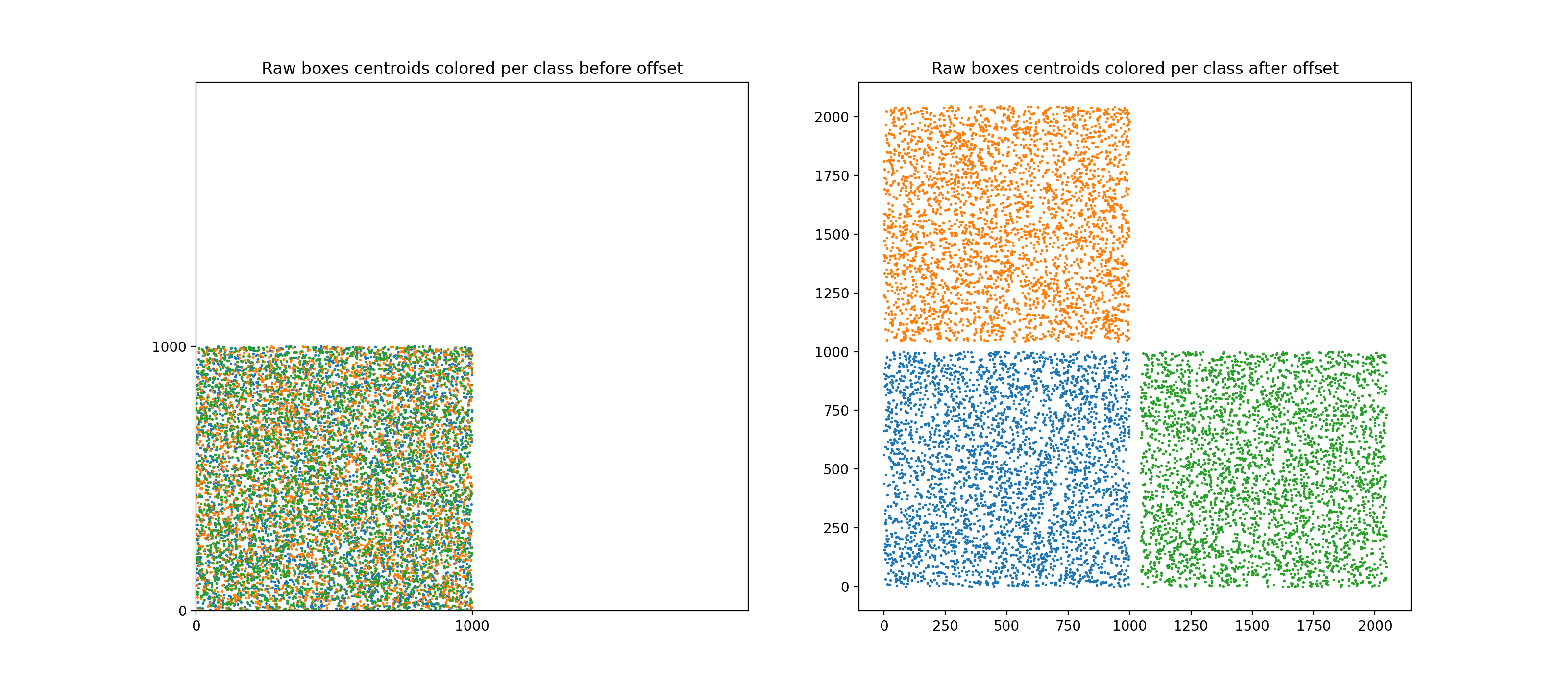
For multiclass support, a peculiar method to offset bounding boxes was used (offseting bounding boxes class-wise is the standard way to apply NMS class-wise). Note that the standard way to offset bboxes is to create a "diagonal per block" aspect, with each class' bboxes being positioned along a virtual diagonal.

Note that this would hurt performances because the underlying RTree that we would build on this would be suboptimal: many regions would actually be empty (because RTree builds rectangular regions) and the query time would be impacted.

Instead, here the boxes are offseted forming a "mosaic" of class-wise regions, see figure below.

Performances

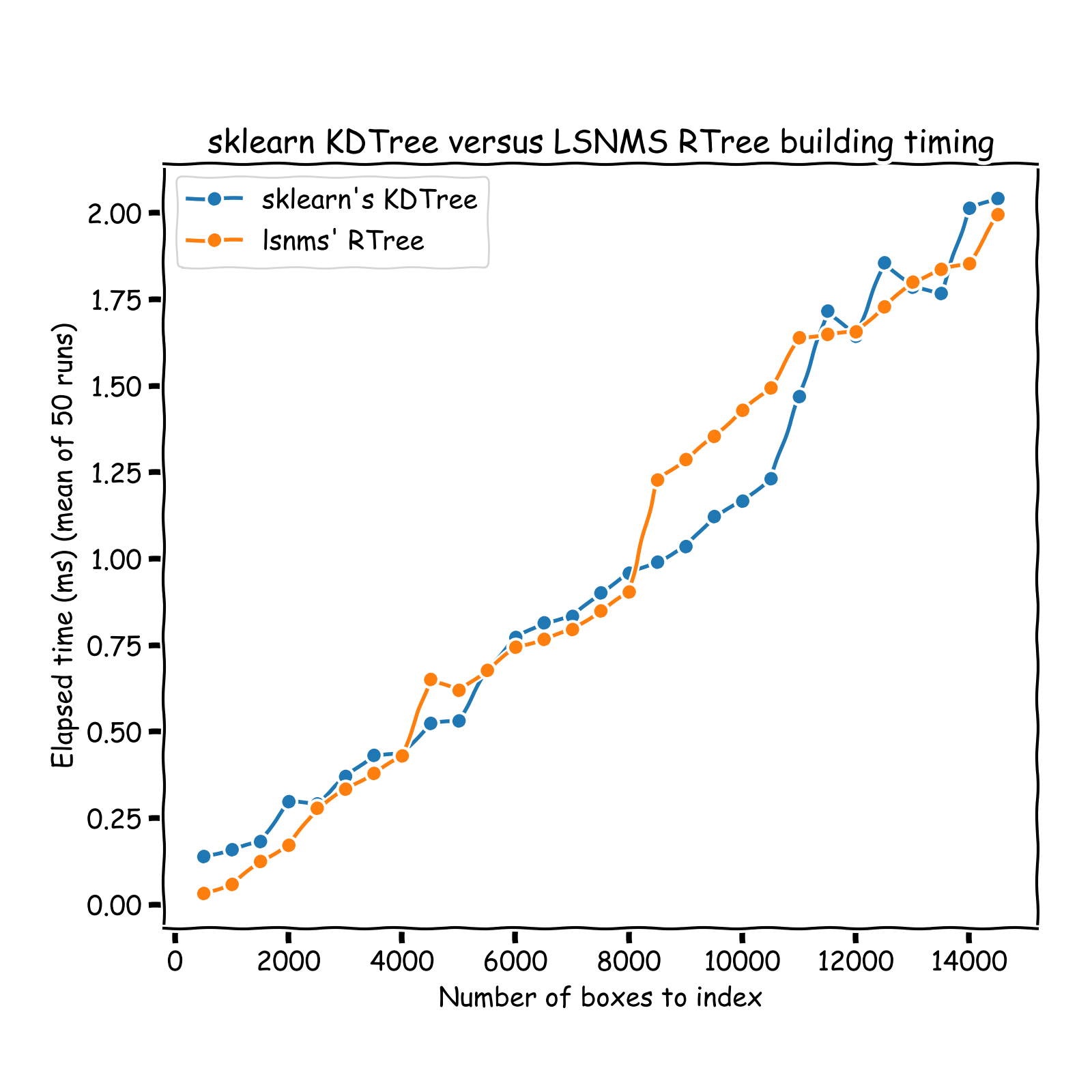
The RTree implemented in this repo was timed against scikit-learn's neighbors one. Note that runtimes are not fair to compare since sklearn implementation allows for node to contain between leaf_size and 2 * leaf_size datapoints. To account for this, I timed my implementation against sklearn tree with int(0.67 * leaf_size) as leaf_size.

Tree building time

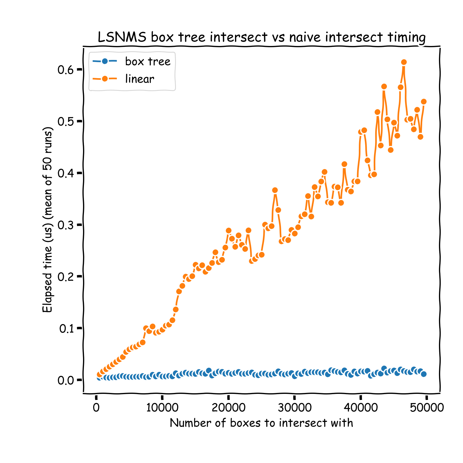
Tree query time