Quantitate liver histopathology in whole slide images

Project description
liverquant
Liverquant is a Python package designed for automated analysis of Whole Slide Images (WSI) to assess Non-alcoholic Fatty Liver Disease (NAFLD) or Metabolic dysfunction Associated Steatotic Liver Disease (MASLD). This toolbox enables the detection of fat globules within image tiles (Example 1) and is directly applicable to WSIs (Example 2). In our evaluation, we utilized this toolbox on a public dataset comprising 109 WSIs. Additionally, the toolbox facilitates fibrosis estimation, demonstrated in Example 3 and Example 4. Future plans involve expanding its capabilities to quantify inflammation and ballooning.
Contents
Installation
The recommended way to install is via pip:
pip install liverquant
Fat Quantification
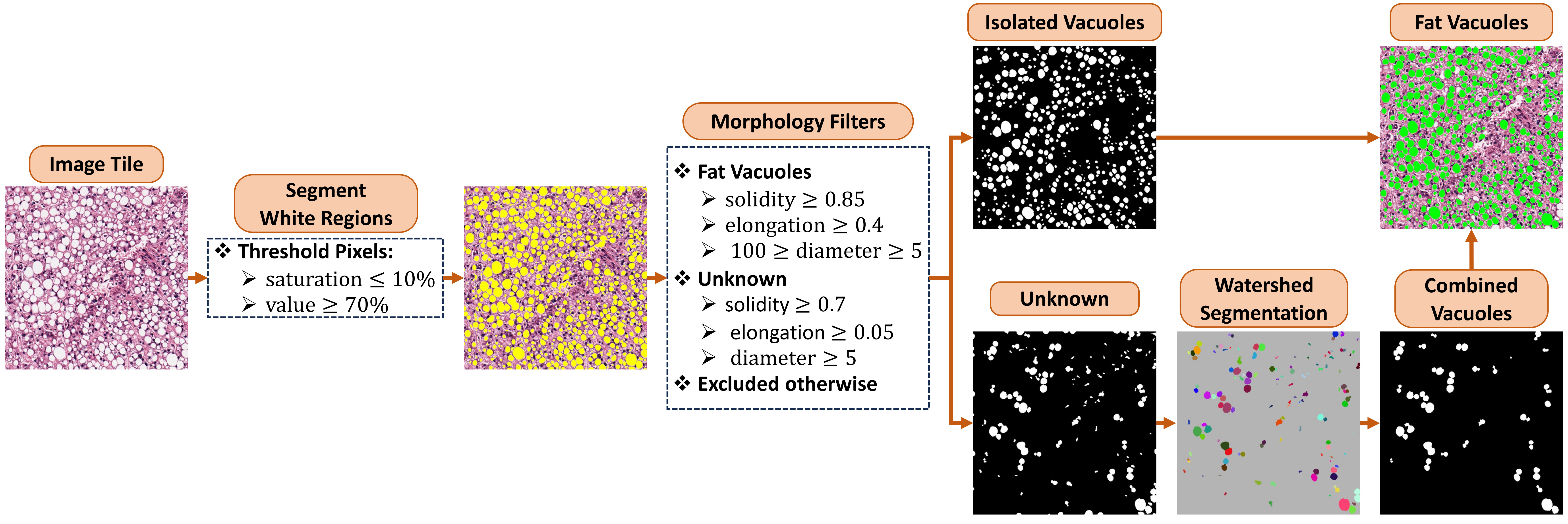
In liver pathology, the presence of fat can be indicative of various conditions, such as fatty liver disease (steatosis), which can occur in the context of alcohol abuse, obesity, diabetes, or metabolic syndrome. Hematoxylin and Eosin (H&E) staining is a widely used technique in pathology that provides basic information about tissue architecture and cellular morphology. Under H&E staining, lipids (fats) appear as clear or pale vacuoles within cells. The workflow to identify fat vacuoles is shown below. In brief, white regions are segmented using Hue-Saturation-Value channels. Isolated fat vacuoles are segmented using morphological features. Overlapping fat globules are separated using a watershed segmentation and then identified using the same filters applied to isolated fat vacuoles.
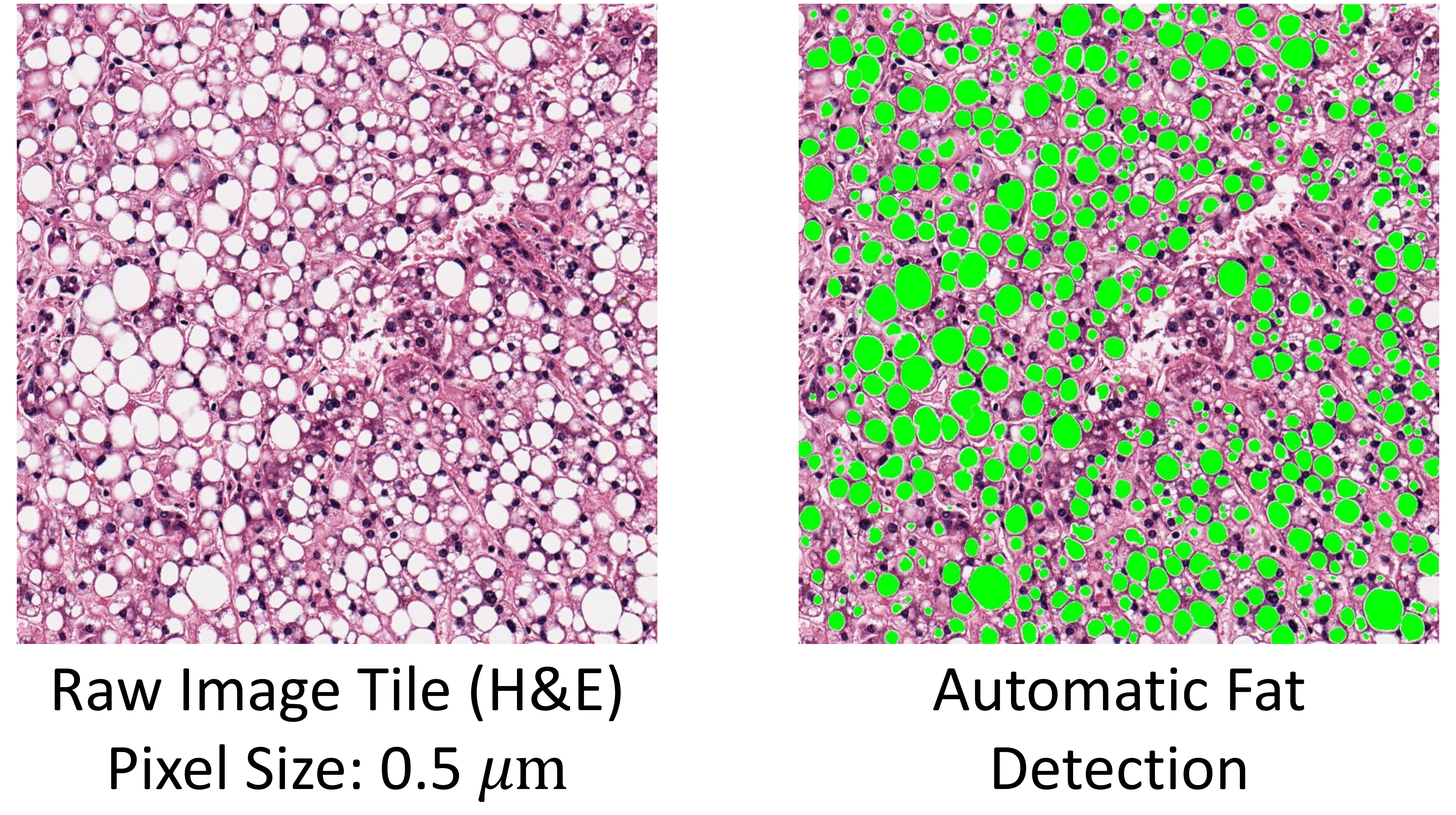
Note: The image tile used in this example is downloaded from histology page with the tissue sample ID GTEX-12584-1526.
The library implements two main methods to identify fat globules.
detect_fat_globules
Retrieve a binary mask for fat vacuoles from input RGB image tile.
- Parameters:
- img: {numpy.ndarray}: input RGB image tile in range [0, 255]
- mask: {numpy.ndarray}: binary mask (either 0 or 255) for regions-of-interest [default=None]
- lowerb: {list: 3}: inclusive lower bound array in HSV-space for color segmentation [default=[0, 0, 200]]
- upperb: {list: 3}: inclusive upper bound array in HSV-space for color segmentation [default=[180, 25, 255]]
- overlap: {int}: globules with centre inside overlap region will be excluded to avoid double-counting in whole-slide-image [default=0]
- resolution: {float}: pixel size in micro-meter [default=1]
- min_diameter: {float}: minimum diameter of a white blob to be considered as a fat globule [default=5]
- max_diameter: {float}: maximum diameter of a white blob to be considered as a fat globule [default=100]
- Returns:
- mask: {numpy.ndarray}: binary mask (either 0 or 255) for identified fat vacuoles
For color segmentation, you must provide the lower and upper bounds for Hue-Saturation-Value channels. Note that similar to OpenCV, Hue has values from 0 to 180, Saturation and Value from 0 to 255. To pick the white color, Saturation between 0 and 25 is filtered out by default. Overlapping fat globules are separated using a watershed segmentation. Fat globules are then identified by filtering blobs based on morphological features including size, solidity, and elongation.
Example 1
Here is a short script to demonstrate the utility of detect_fat_globules.
import cv2 as cv
from liverquant import detect_fat_globules

# read sample image tile
img = cv.imread('./example/tile01_HE.jpg')
img = cv.cvtColor(img, cv.COLOR_BGR2RGB)

# Detect globules
mask = detect_fat_globules(img, resolution=0.4942)

# Tag globules with green color
img[mask == 255, :] = [5, 255, 5]

# write the tagged image
cv.imwrite('./example/tile01_HE_tagged.jpg', cv.cvtColor(img, cv.COLOR_BGR2RGB))
detect_fat_globules_wsi
Retrieve fat vacuoles in cv2geojson.GeoContour format from the whole slide image (WSI).
- Parameters:
- slide: {openslide}: A handle object to the whole slide image
- roi: {list: cv2geojson.GeoContours}: regions-of-interest in the WSI frame [default=None]
- lowerb: {list: 3}: inclusive lower bound array in HSV-space for color segmentation [default=[0, 0, 200]]
- upperb: {list: 3}: inclusive upper bound array in HSV-space for color segmentation [default=[180, 25, 255]]
- tile_size: {int}: the tile size to sweep the whole slide image [default=2048]
- overlap: {int}: globules with centre inside overlap region will be excluded to avoid double-counting in whole-slide-image [default=128]
- downsample: {int}: downsampling ratio as a power of two [default=2]
- min_diameter: {float}: minimum diameter of a white blob to be considered as a fat globule [default=5]
- max_diameter: {float}: maximum diameter of a white blob to be considered as a fat globule [default=100]
- cores_num: {int}: max number of cores to be used for parallel computation
- Returns:
- fat_proportion_area: {float}: the amount of fat in the tissue represented in percent
- vacoules: {list: cv2geojson.GeoContour}: polygons representing fat vacoules
- roi: {list: cv2geojson.GeoContour}: same as input roi if provided; otherwise, representing the foreground mask
- run_time: {float}: run time for the code completion in seconds
This function divides the input image into overlapping image tiles and applies the
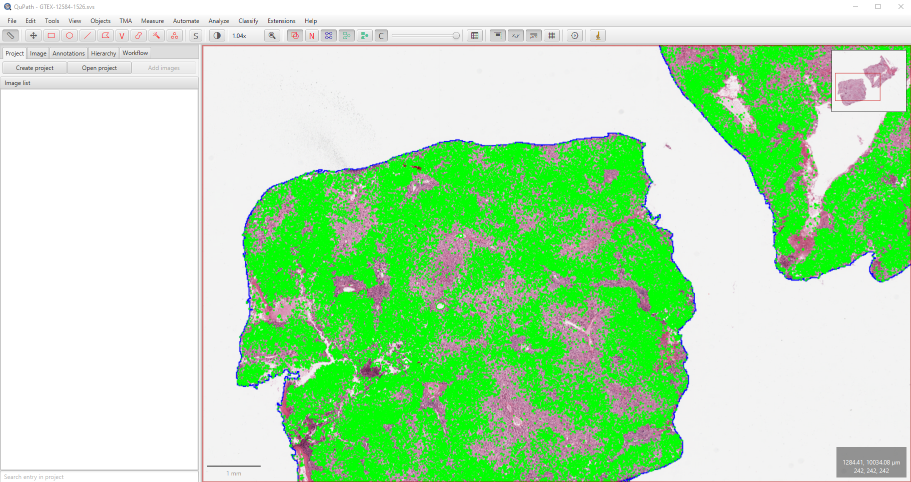
detect_fat_globulesalgorithm (refer to Example 1) to each image tile.detect_fat_globules_wsiemploys parallel computation, and the entire script should be enclosed within aif __name__ == '__main__'block. Liverquant export detected geometrical features in geojson format using thecv2geojsonpython package, which can be visualised using dedicated software tools like QuPath.
Example 2
Here is a short script to demonstrate the utility of detect_fat_globules_wsi. The WSI used in this example is not provided due to its large size but can be downloaded from histology page with the tissue sample ID GTEX-12584-1526. The estimated fat proportionate area is 13.8% and the run time was about 214 seconds.
from liverquant import detect_fat_globules_wsi
from cv2geojson import export_annotations
from openslide import OpenSlide

if __name__ == '__main__':
    # open the whole slide image
    slide = OpenSlide('./example/GTEX-12584-1526.svs')

    # detect fat globules
    fat_proportionate_area, globules, roi, run_time = detect_fat_globules_wsi(slide, cores_num=12)

    # export geojson features
    features = []
    for geocontour in roi:
        features.append(geocontour.export_feature(color=(0, 0, 255), label='foreground'))
    for geocontour in globules:
        features.append(geocontour.export_feature(color=(0, 255, 0), label='fat'))
    export_annotations(features, './example/GTEX-12584-1526.geojson')

    # print out results
    print(f'The fat proportionate area is {fat_proportionate_area}%.')
    print(f'The run time is {run_time} seconds.')
Genotype-Tissue Expression (GTEx) public dataset
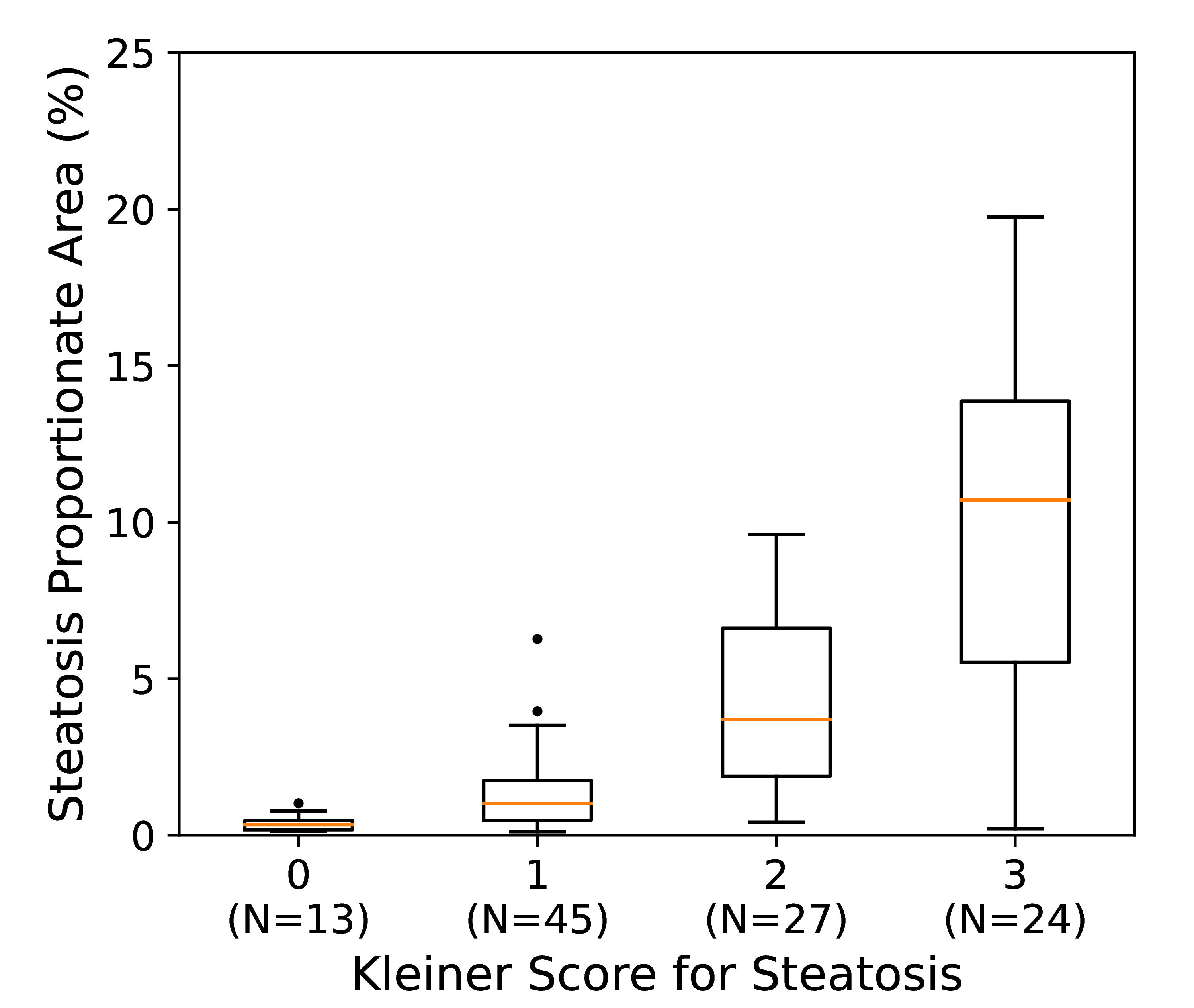
Our validation process for the steatosis quantification algorithm involved analyzing H&E whole slide images from the Genotype-Tissue Expression (GTEx) public portal, sourced from the diverse collection of histology images obtained from various tissue types in postmortem donors. Out of the 262 liver biopsy cases selected for this study, exhibiting steatosis, Kleiner scores were automatically extracted from pathology notes for 109 cases. This extraction involved scanning pathology notes to assess the steatosis proportionate area (SPA), categorized into four groups: 0 (SPA≤5), 1 (5<SPA≤33), 2 (33<SPA≤66), and 3 (66<SPA). For convenient access, the list of these 109 slides can be downloaded [here].
To evaluate the steatosis quantification algorithm, we analysed an external public dataset of H&E whole slide images from the Genotype-Tissue Expression (GTEx) public portal (Broad Institute, Cambridge, MA, USA). The GTEx tissue image repository includes a diverse collection of histology images derived from various tissue types obtained from postmortem donors. Out of the 262 liver biopsy cases selected for this study, exhibiting steatosis, Kleiner scores were automatically extracted from pathology notes for 109 cases. To achieve this, pathology notes were scanned for the steatosis proportionate area (SPA) and then categorised into four groups: 0 (SPA≤5), 1 (5<SPA≤33), 2 (33<SPA≤66), and 3 (66<SPA). For convenient access, the list of these 109 slides can be downloaded here. The correlation between estimated SPA at 20x magnification and extracted Kleiner scores is visually represented in the box-and-whisker plot below, showing a moderate Spearman rank correlation (ρ=0.75) within this subset of N=109 cases.
You can access and download the slides using the following Python script:
import requests
from pathlib import Path
import pandas as pd

# define the local working directory
root_path = Path('.\\Example')
path_to_dataset = root_path / 'gtex_liver_steatosis_dataset.csv'
df = pd.read_csv(path_to_dataset)


def download_file(url, destination):
    try:
        response = requests.get(url, stream=True)
        response.raise_for_status()

        with open(destination, 'wb') as file:
            for chunk in response.iter_content(chunk_size=8192):
                if chunk:
                    file.write(chunk)

        print(f"File downloaded to {destination}")
    except requests.exceptions.RequestException as e:
        print(f"An error occurred: {e}")


if __name__ == "__main__":
    # create a folder to store whole slide images
    path_to_slides = root_path / 'slides'
    if not path_to_slides.is_dir():
        path_to_slides.mkdir()

    # download the slides
    for i in range(df.shape[0]):
        slide_name = df['Slide ID'][i]
        file_url = "https://brd.nci.nih.gov/brd/imagedownload/{}".format(slide_name)
        destination_file = path_to_slides / '{}.svs'.format(slide_name)

        if not destination_file.is_file():
            print(f'downloading {file_url}...')
            download_file(file_url, destination_file)
Upon downloading the slides, utilize the script below to compute the steatosis proportionate area (SPA).
from pathlib import Path
import pandas as pd
from liverquant import detect_fat_globules_wsi
import numpy as np
from openslide import OpenSlide

root_path = Path('.\\Example') # local working directory
path_to_slides = root_path / 'slides'
path_to_dataset = root_path / 'gtex_liver_steatosis_dataset.csv'

if __name__ == '__main__':
    df = pd.read_csv(path_to_dataset)
    for index in range(df.shape[0]):
        slide_id = df['Slide ID'][index]
        slide_filename = path_to_slides / '{}.svs'.format(slide_id)

        slide = OpenSlide(slide_filename)
        spa, contours, roi, run_time = detect_fat_globules_wsi(slide,
                                                               upperb=[180, 25, 255],
                                                               lowerb=[0, 0, 200],
                                                               tile_size=2048,
                                                               overlap=128,
                                                               downsample=1,
                                                               min_diameter=5,
                                                               max_diameter=100,
                                                               cores_num=12)

        # store results
        df.at[index, 'SPA'] = np.round(spa, 2)
        df.at[index, 'Runtime'] = np.round(run_time, 3)
        print(f'slide {slide_id}--- fpa: {spa}  run time:{run_time}')
    df.to_csv(path_to_dataset, index=False)
Fibrosis Quantification
Liver fibrosis is a progressive condition characterized by the excessive accumulation of extracellular matrix components, particularly collagen, within the liver tissue. It is typically a consequence of chronic liver injury caused by various factors such as viral hepatitis, alcohol abuse, metabolic disorders, or autoimmune diseases. The excessive collagen deposition disrupts the normal liver architecture and impairs its function over time.
To evaluate the extent of liver fibrosis, histological staining techniques are commonly employed. Picrosirius red (PSR), Masson's Trichrome (MTC), and Van Gieson (VG) staining are three widely used methods to visualize and quantify the collagen content within liver tissue. These techniques allow for the identification of collagen fibers and provide valuable information about the severity and distribution of fibrosis.
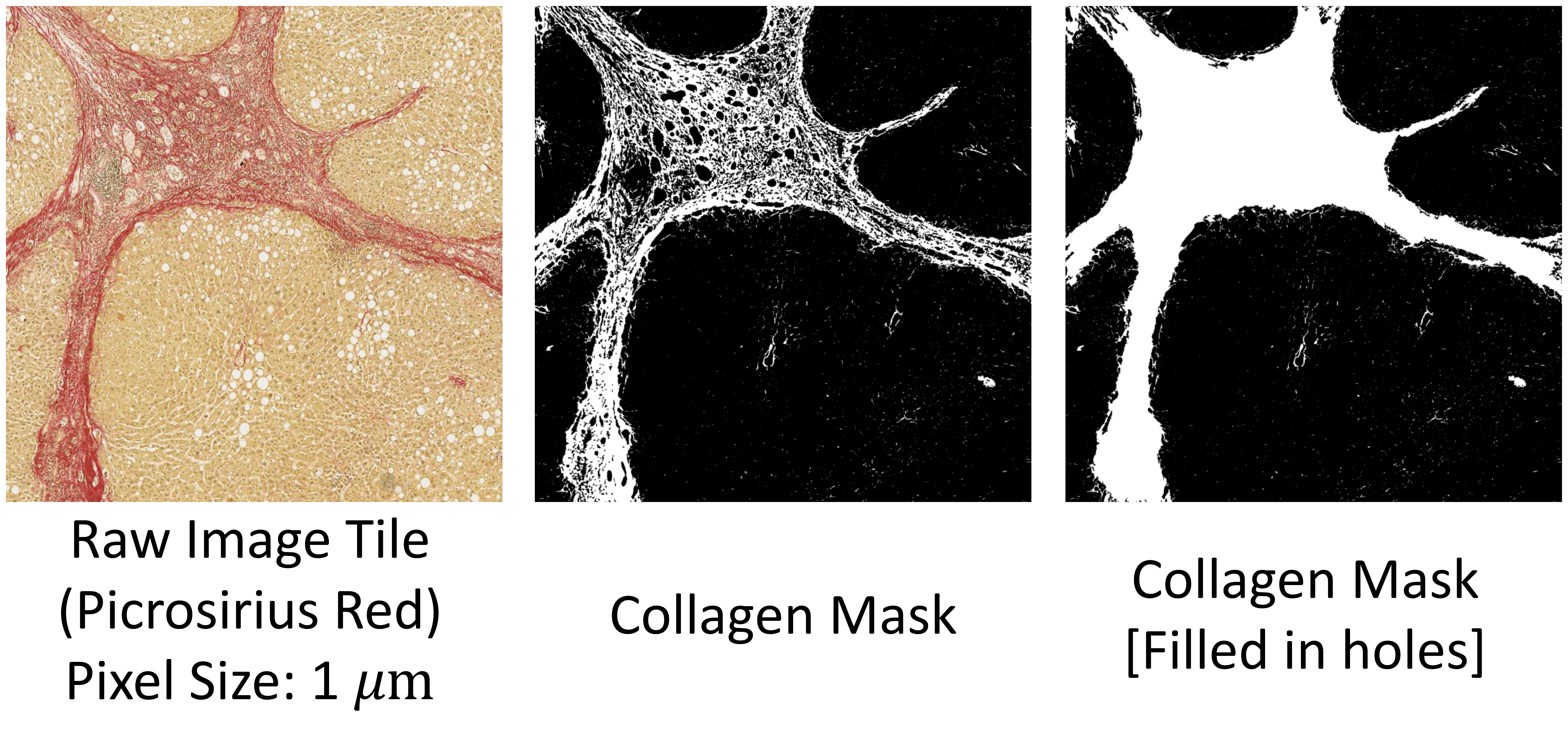
1- Picrosirius red (PSR) staining: PSR staining specifically highlights collagen fibers and helps differentiate between mature (thick, red-orange staining) and immature (thin, green staining) collagen. This staining technique allows for the assessment of collagen distribution, fiber thickness, and the presence of newly formed collagen.
2- Masson's Trichrome (MTC) staining: MTC staining is a widely used technique to visualize collagen fibers in tissues. It involves staining collagen fibers blue or green, nuclei dark blue or black, and cytoplasm and muscle fibers red. Collagen fibers appear as blue-green structures, allowing for the identification and quantification of fibrosis. MTC staining provides information about the extent of collagen deposition and can help evaluate fibrosis severity.
3- Van Gieson (VG) staining: VG staining is another method widely used to assess collagen deposition in tissues. It stains collagen fibers red or pink, while other tissue components such as muscle fibers, cytoplasm, and nuclei are stained yellow or brown. This staining technique allows for the identification and quantification of collagen within the liver tissue, enabling the evaluation of fibrosis severity.
The library implements two main methods to identify collagens using colour segmentation in both individual image tiles and the whole slide image.
segment_fibrosis
Retrieve a binary mask for segmented regions based on their colour profile in the HSV space.
-
Parameters:
- img: {numpy.ndarray}: input RGB image tile in range [0, 255]
- mask: {numpy.ndarray}: binary mask (either 0 or 255) for regions-of-interest [default=None]
- stain: {string}: VG or PSR or MTC
- lowerb: {list: 3}: inclusive lower bound array in HSV-space for color segmentation [default=None]
- upperb: {list: 3}: inclusive upper bound array in HSV-space for color segmentation [default=None]
- mixing_matrix: {numpy.ndarray}: the proportion of each wavelength absorbed from red, green, and blue channels [default=None]
- ref_mixing_matrix: {numpy.ndarray}: reference mixing matrix to normalise input image
- scale: {list: 3}: global scaling factor for stain normalisation
- hole_size: {float}: remove holes smaller than hole_size; if zero, all holes are reserved. If -1, all holes will be removed. [default=0]
- blob_size: {float}: remove blobs smaller than blob_size; if zero, all blobs are reserved.
- resolution: {float}: pixel size in micro-meter [default=1]
-
Returns:
- cpa: {float}: Collagen Proportionate Area (CPA) in percent
- collagen_mask: {numpy.ndarray}: binary mask (either 0 or 255) for segmented regions
- roi: {numpy.ndarray}: binary mask (either 0 or 255) for the regions of interest
Note that similar to OpenCV, Hue has values from 0 to 180, Saturation and Value from 0 to 255.
Example 3
Here is a short script to demonstrate the utility of segment_fibrosis. An image tile stained with PSR is provided in the example folder. To segment the collagen shown in red, Hue between 0 and 10 or 170-180 should be filtered out. We have combined the two ranges into one effective range [-10, 10] in the sample code below. Since Hue is inherently periodic, negative Hue can be interpreted as positive integers by adding 180. Note that similar to OpenCV, Hue has values from 0 to 180.
import cv2 as cv
from liverquant import segment_fibrosis

# read sample image tile
img = cv.imread('./example/tile02_PSR.jpg')
img = cv.cvtColor(img, cv.COLOR_BGR2RGB)

cpa, mask, roi = segment_fibrosis(img,
                                  lowerb=[-10, 50, 100],
                                  upperb=[10, 255, 255],
                                  resolution=1.0124)

print(f'CPA = {cpa}%')

# write the tagged image
cv.imwrite('./example/tile02_PSR_mask.jpg', mask)
segment_fibrosis_wsi
Retrieve segmented regions in cv2geojson.GeoContour format based on their colour profile in the HSV space from the whole slide image (WSI).
-
Parameters:
-
img: {numpy.ndarray}: input RGB image tile in range [0, 255]
-
stain: {string}: VG or PSR or MTC
-
roi: {list: cv2geojson.GeoContours}: regions-of-interest in the WSI frame [default=None]
-
lowerb: {list: 3}: inclusive lower bound array in HSV-space for color segmentation [default=None]
-
upperb: {list: 3}: inclusive upper bound array in HSV-space for color segmentation [default=None]
-
mixing_matrix: {numpy.ndarray}: the proportion of each wavelength absorbed from red, green, and blue channels [default=None]
-
ref_mixing_matrix: {numpy.ndarray}: reference mixing matrix to normalise input image
-
scale: {list: 3}: global scaling factor for stain normalisation
-
hole_size: {float}: remove holes smaller than hole_size; if zero, all holes will be reserved. If -1, all holes will be removed. [default=0]
-
blob_size: {float}: remove blobs smaller than blob_size; if zero, all blobs are reserved [default=0]
-
tile_size: {int}: the tile size to sweep the whole slide image [default=2048]
-
downsample: {int}: downsampling ratio as a power of two [default=2]
-
cores_num: {int}: max number of cores to be used for parallel computation [default=4]
-
-
Returns:
- cpa: {float}: Collagen Proportionate Area (CPA) in percent
- geocontours: {list: cv2geojson.GeoContour}: polygons representing segmented fibrotic regions
- roi: {numpy.ndarray}: binary mask (either 0 or 255) for the regions of interest
Note that similar to OpenCV, Hue has values from 0 to 180, Saturation and Value from 0 to 255. This function divides the input image into image tiles and applies the
segment_by_coloralgorithm (refer to Example 3) to each image tile.segment_by_color_wsiemploys parallel computation, and the entire script should be enclosed within aif __name__ == '__main__'block. Liverquant export detected geometrical features in geojson format using thecv2geojsonpython package, which can be visualised using dedicated software tools like QuPath.
Example 4
Here is a short script to demonstrate the utility of segment_fibrosis_wsi. To segment the collagen shown in red, Hue between 0 and 10 or 170-180 should be filtered out. Since Hue is inherently periodic, negative Hue can be interpreted as positive integers by adding 180. We have combined the two ranges into one effective range [-10, 10]in the sample code below.
from liverquant import segment_fibrosis_wsi
from cv2geojson import export_annotations
from openslide import OpenSlide

if __name__ == '__main__':
    # open the whole slide image
    slide = OpenSlide('./example/PSR_slide.svs')

    # Segment collagen using Hue-Saturation-Value channels
    cpa, geocontours, roi = segment_fibrosis_wsi(slide,
                                                 stain='PSR',
                                                 lowerb=[-10, 50, 100],
                                                 upperb=[10, 255, 255],
                                                 downsample=16,
                                                 tile_size=4096,
                                                 cores_num=12)

    # print out results
    print(f'The collagen proportionate area is {cpa}%.')

    # export geojson features
    features = []
    for geocontour in roi:
        features.append(geocontour.export_feature(color=(255, 0, 0), label='foreground'))
    for geocontour in geocontours:
        features.append(geocontour.export_feature(color=(0, 0, 255), label='fibrosis'))
    export_annotations(features, './example/PSR_slide.geojson')


Download files
Download the file for your platform. If you're not sure which to choose, learn more about installing packages.
Source Distribution
Built Distribution
Hashes for liverquant-0.0.4-py3-none-any.whl
| Algorithm | Hash digest | |
|---|---|---|
| SHA256 | b01175b4ba2495635350b0e49c286627f3b4e85359d4b8ed6102b233c3a90abd |
|
| MD5 | 404bb94c404d853f5a4387bb0021799a |
|
| BLAKE2b-256 | c50dc886a9ac3636422a2af8484ebb5f812954e16a840d28bbe71265b1ce7c7d |


