Project is devoted to pick waves that are the first to be detected on a seismogram with neural network (CUDA accelerated)

Project description
FirstBreaksPicking
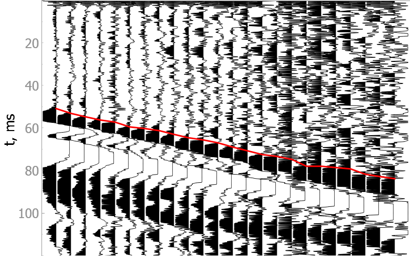
This project is devoted to pick waves that are the first to be detected on a seismogram (first breaks, first arrivals). Traditionally, this procedure is performed manually. When processing field data, the number of picks reaches hundreds of thousands. Existing analytical methods allow you to automate picking only on high-quality data with a high signal / noise ratio.
As a more robust algorithm, it is proposed to use a neural network to pick the first breaks. Since the data on adjacent seismic traces have similarities in the features of the wave field, we pick first breaks on 2D seismic gather, not individual traces.
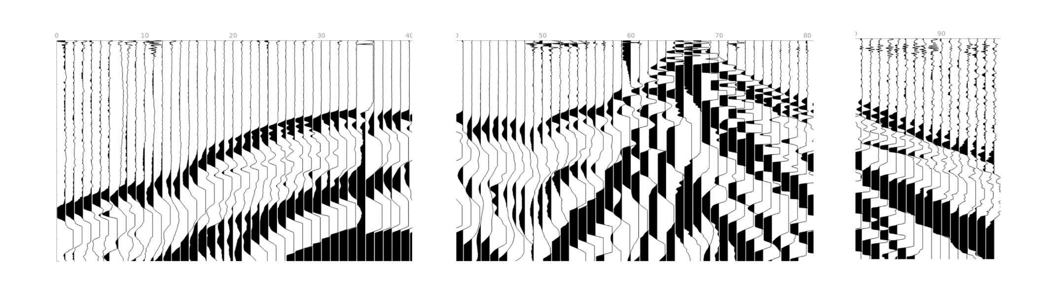
Examples
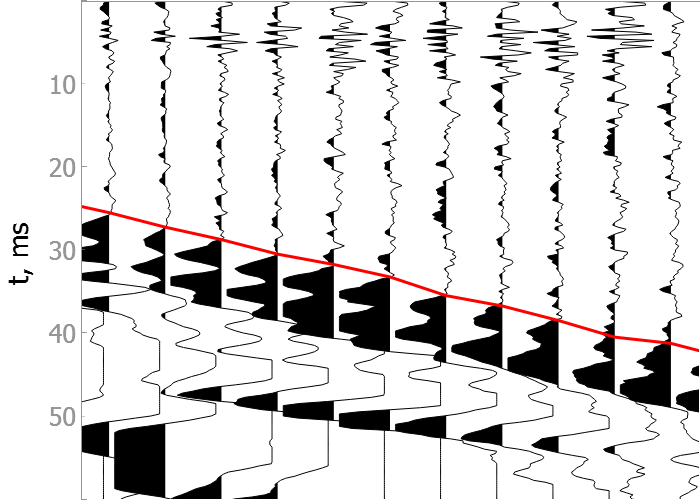
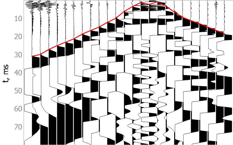
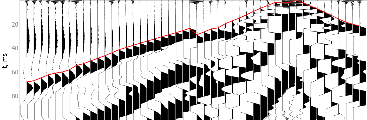
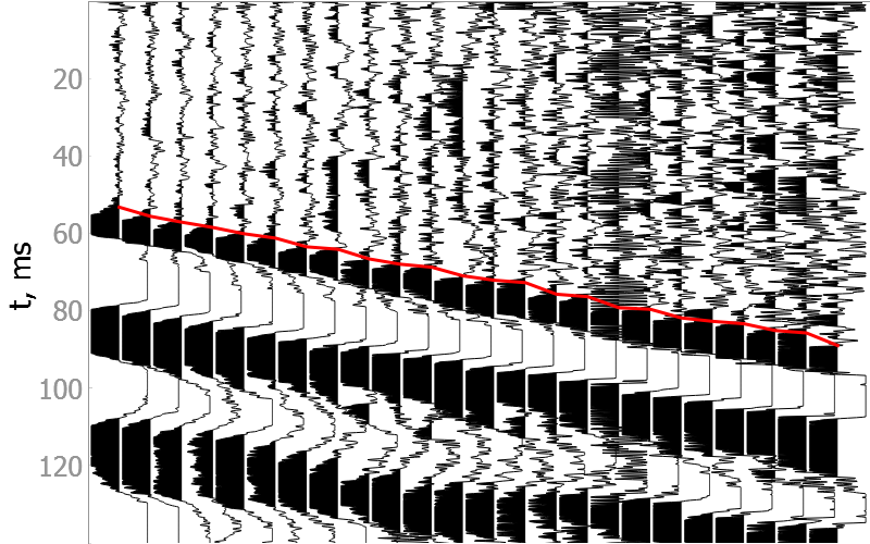
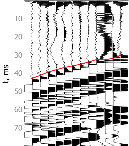
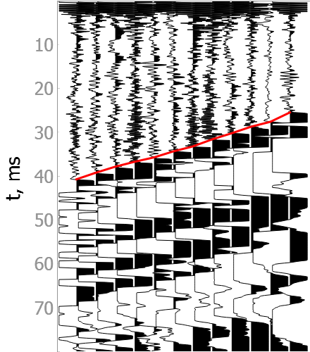
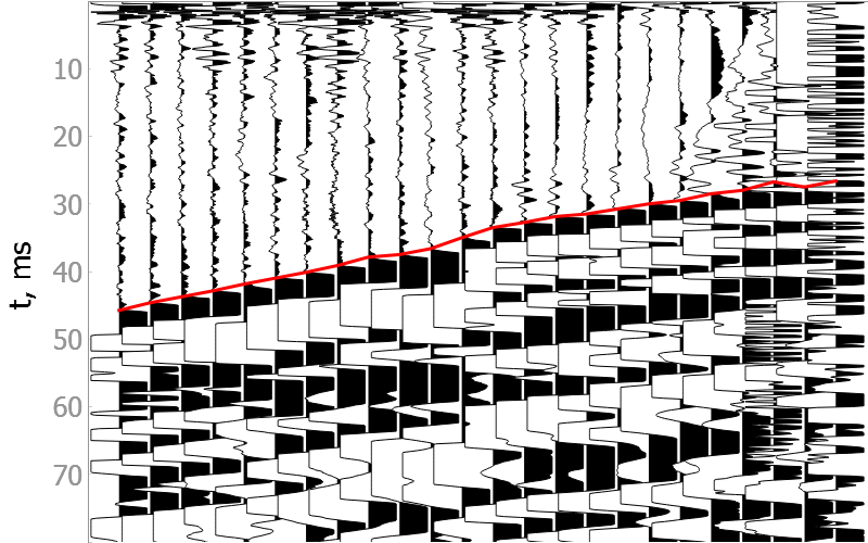
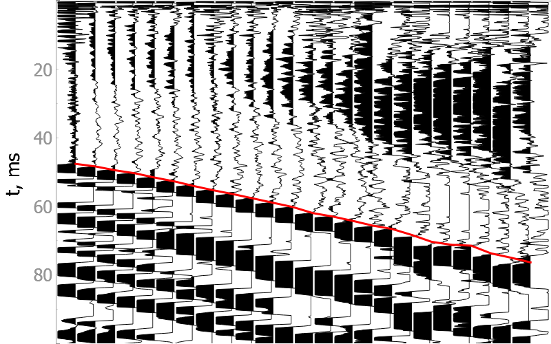
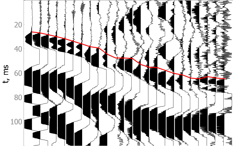
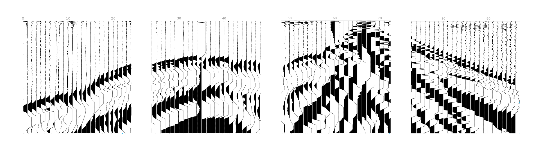
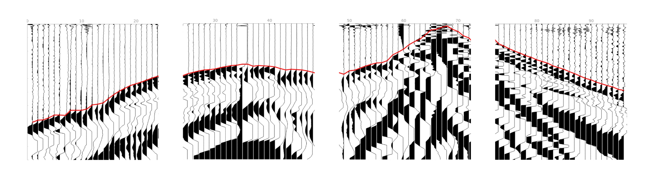
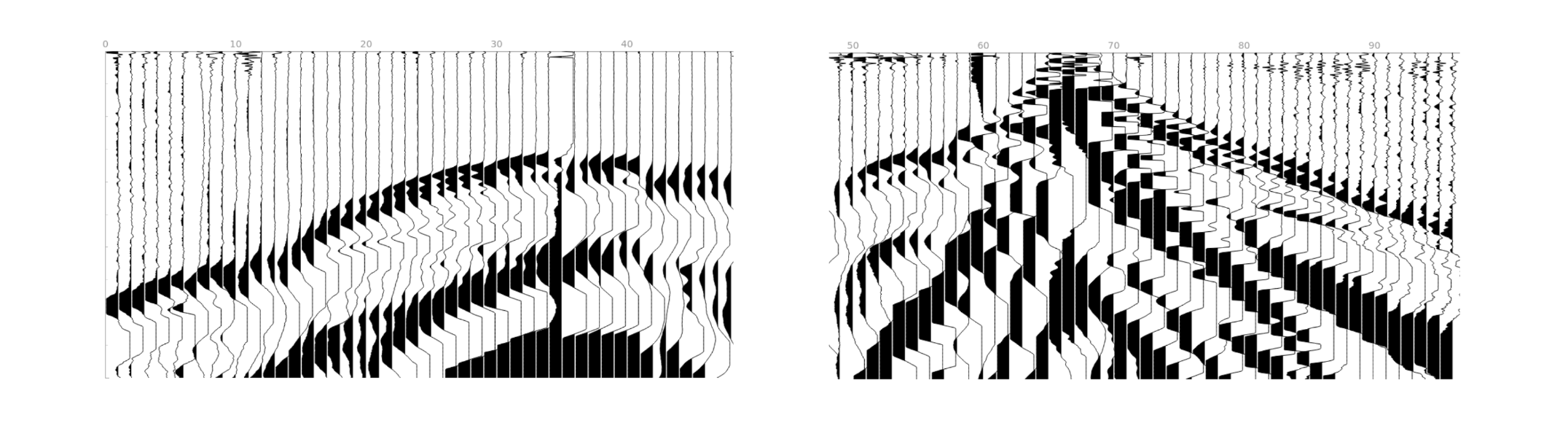
In the drop-down menus below you will find examples of our model picking on good quality data as well as noisy ones.
It is difficult to validate the quality of the model on noisy data, but they show the robustness of the model to various types of noise.
Good quality data
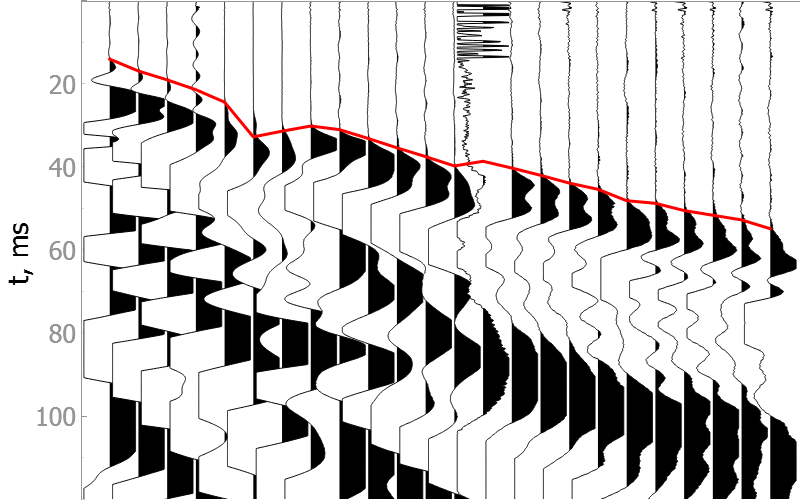
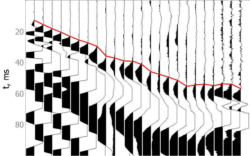
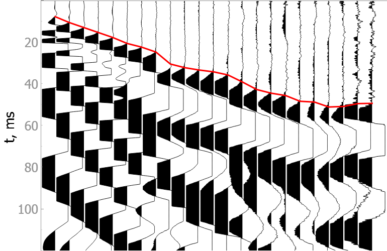
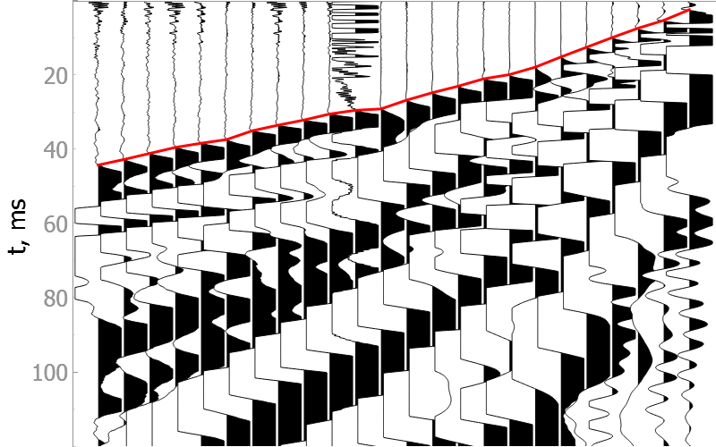

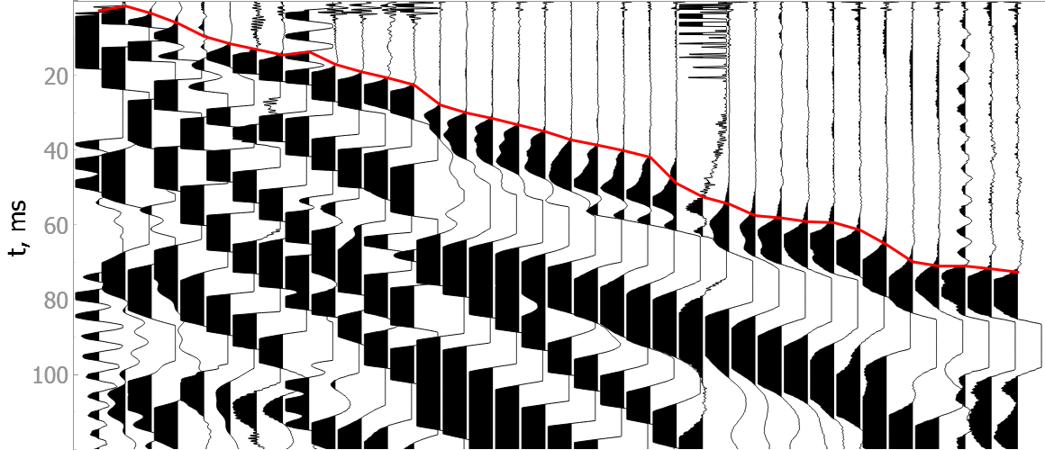
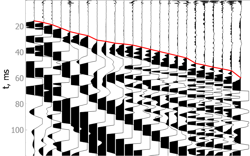
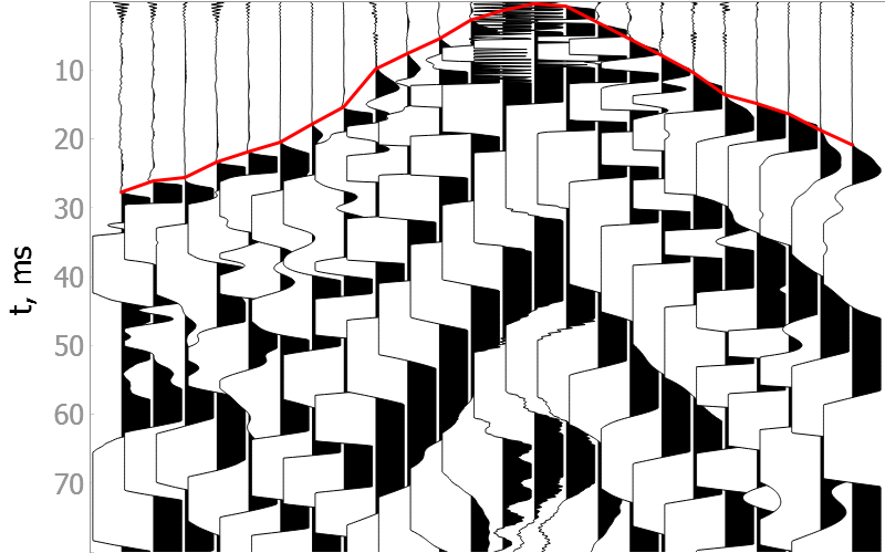
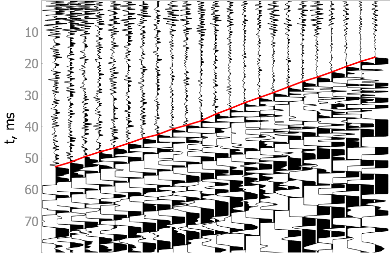
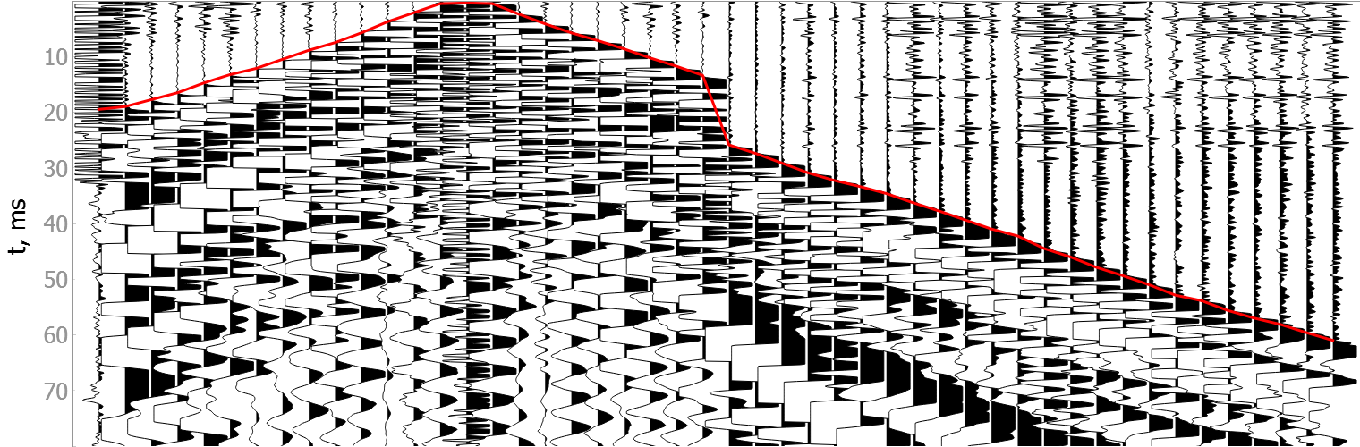
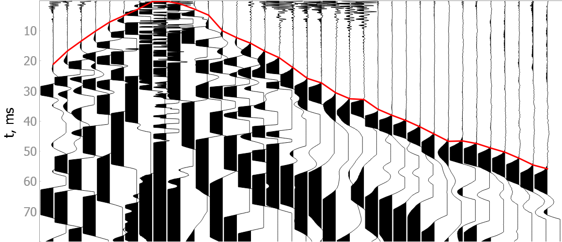
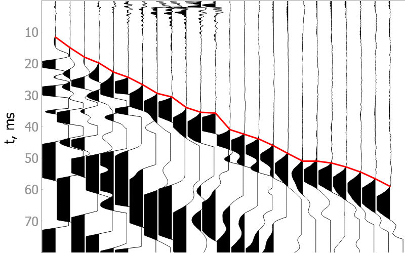
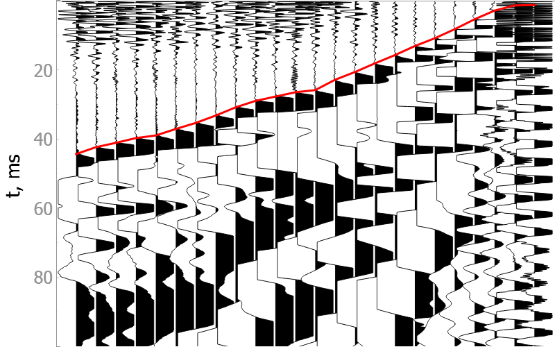
Noisy data
How model was trained?
Model training is described in detail here in the previous version of the project README.
The latest model was trained similarly, but:
- Real land seismic data is used instead of synthetic data.
- UNet3+ model is used, instead of the vanilla UNet.
Installation
Library is available in PyPI:
pip install -U first-breaks-picking
GPU support
You can use the capabilities of GPU (discrete, not integrated with CPU) to significantly reduce picking time. Before started, check here that your GPU is CUDA compatible.
Install GPU supported version of library:
pip install -U first-breaks-picking-gpu
The following steps are operating system dependent and must be performed manually:
- Install latest NVIDIA drivers.
- Install CUDA toolkit. The version must be between 11.x, starting with 11.6. Version 12 also may work, but versions >=11.6 are recommended.
- Install ZLib and CuDNN: Windows and Linux.
Compiled desktop application
Compiled executable files (.exe in .zip archives), as well as installers (.msi), can be downloaded in the Releases section.
If you want to use the capabilities of your dedicated GPU, also follow the steps in the previous step to install the driver, CUDA, CuDNN, and ZLib.
You can run the desktop application on other operating systems (Linux, MacOS) as well, but it must be run using the Python environment.
Extra data
-
To pick first breaks you need to download model.
-
If you have no seismic data, you can also download small SGY file.
It's also possible to download them with Python using the following snippet:
from first_breaks.utils.utils import (download_demo_sgy,
                                      download_model_onnx)

sgy_filename = 'data.sgy'
model_filename = 'model.onnx'

download_demo_sgy(sgy_filename)
download_model_onnx(model_filename)
How to use it
The library can be used in Python, or you can use the desktop application.
Python
Programmatic way has more flexibility for building your own picking scenario and processing multiple files.
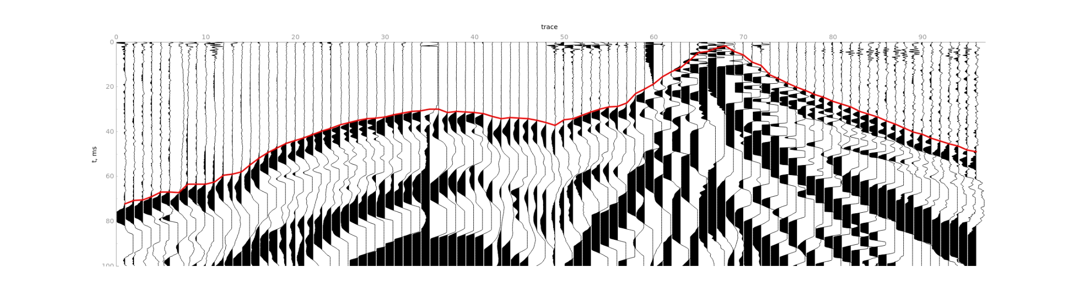
Minimal example
The following snippet implements the picking process of the demo file. As a result, you can get an image from the project preview.
from first_breaks.utils.utils import download_demo_sgy
from first_breaks.sgy.reader import SGY
from first_breaks.picking.task import Task
from first_breaks.picking.picker_onnx import PickerONNX
from first_breaks.desktop.graph import export_image

sgy_filename = 'data.sgy'
download_demo_sgy(fname=sgy_filename)
sgy = SGY(sgy_filename)

task = Task(source=sgy_filename,
            traces_per_gather=12,
            maximum_time=100,
            gain=2)
picker = PickerONNX()
task = picker.process_task(task)

# create an image with default parameters
image_filename = 'default_view.png'
export_image(task, image_filename)

# create an image from the project preview
image_filename = 'project_preview.png'
export_image(task, image_filename,
             time_window=(0, 60),
             traces_window=(79.5, 90.5),
             show_processing_region=False,
             headers_total_pixels=80,
             height=500,
             width=700,
             hide_traces_axis=True)
For a better understanding of the steps taken, expand and read the next section.
Detailed examples
Show examples
Download demo SGY
Let's download the demo file. All the following examples assume that the file is downloaded and saved as data.sgy.
You can also put your own SGY file.
from first_breaks.utils.utils import download_demo_sgy

sgy_filename = 'data.sgy'
download_demo_sgy(fname=sgy_filename)
Create SGY
We provide several ways to create SGY object: from file, bytes or numpy array.
From file:
from first_breaks.sgy.reader import SGY

sgy_filename = 'data.sgy'
sgy = SGY(sgy_filename)
From bytes:
from first_breaks.sgy.reader import SGY

sgy_filename = 'data.sgy'

with open(sgy_filename, 'rb') as fin:
    sgy_bytes = fin.read()

sgy = SGY(sgy_bytes)
If you want to create from numpy array, extra argument dt_mcs is required:
import numpy as np
from first_breaks.sgy.reader import SGY

num_samples = 1000
num_traces = 48
dt_mcs = 1e3

traces = np.random.random((num_samples, num_traces))
sgy = SGY(traces, dt_mcs=dt_mcs)
Content of SGY
Created SGY allows you to read traces, get observation parameters and view headers (empty if created from numpy)
from first_breaks.sgy.reader import SGY

sgy_filename = 'data.sgy'
sgy = SGY(sgy_filename)

# get all traces or specific traces limited by time
all_traces = sgy.read()
block_of_data = sgy.read_traces_by_ids(ids=[1, 2, 3, 10],
                                       min_sample=100,
                                       max_sample=500)

# number of traces, values are the same
print(sgy.num_traces, sgy.ntr)
# number of time samples, values are the same
print(sgy.num_samples, sgy.ns)
# = (ns, ntr)
print(sgy.shape)
# time discretization, in mcs, in mcs, in ms, fs in Hertz
print(sgy.dt, sgy.dt_mcs, sgy.dt_ms, sgy.fs)

# dict with headers in the first 3600 bytes of the file
print(sgy.general_headers)
# pandas DataFrame with headers for each trace
print(sgy.traces_headers.head())
Create task for picking
Next, we create a task for picking and pass the picking parameters to it. They have default values, but for the
best quality, they must be matched to specific data. You can use the desktop application to evaluate the parameters.
A detailed description of the parameters can be found in the Picking process chapter.
from first_breaks.sgy.reader import SGY
from first_breaks.picking.task import Task

sgy_filename = 'data.sgy'
sgy = SGY(sgy_filename)

task = Task(source=sgy,
            traces_per_gather=24,
            maximum_time=200)
Create Picker
In this step, we instantiate the neural network for picking. If you downloaded the model according to the installation section, then pass the path to it. Or leave the path to the model empty so that we can download it automatically.
It's also possible to use GPU/CUDA to accelerate computation. By default cuda is selected if you have finished
all steps regarding GPU in Installation section. Otherwise, it's cpu.
You can also set the value of parameter batch_size, which can further speed up the calculations on the GPU.
However, this will require additional video memory (VRAM).
NOTE: When using the CPU, increasing batch_size does not speed up the calculation at all, but it may
require additional memory costs (RAM). So don't increase this parameter when using CPU.
from first_breaks.picking.picker_onnx import PickerONNX

# the library will determine the best available device
picker_default = PickerONNX()

# create picker explicitly on CPU
picker_cpu = PickerONNX(device='cpu')

# create picker explicitly on GPU
picker_gpu = PickerONNX(device='cuda', batch_size=2)

# transfer model to another device
picker_cpu.change_settings(device='cuda', batch_size=3)
picker_gpu.change_settings(device='cpu', batch_size=1)
Pick first breaks
Now, using all the created components, we can pick the first breaks and export the results.
from first_breaks.picking.task import Task
from first_breaks.picking.picker_onnx import PickerONNX
from first_breaks.sgy.reader import SGY

sgy_filename = 'data.sgy'
sgy = SGY(sgy_filename)

task = Task(source=sgy,
            traces_per_gather=24,
            maximum_time=200)
picker = PickerONNX()
task = picker.process_task(task)

# you can see results of picking
print(task.picks_in_samples)
print(task.picks_in_ms)
print(task.confidence)

# you can export picks to file as plain text
task.export_result_as_txt('result.txt')
# or save as json file
task.export_result_as_json('result.json')
# or make a copy of source SGY and put picks to 236 byte
task.export_result_as_sgy('result.segy',
                          byte_position=236,
                          encoding='i',
                          picks_unit='mcs')
Visualizations
You can save the seismogram and picks as an image. We use Qt backend for visualizations. Here we describe some usage scenarios.
We've added named arguments to various scenarios for demonstration purposes, but in practice you can use them all. See the function arguments for more visualization options.
Plot SGY only:
from first_breaks.sgy.reader import SGY
from first_breaks.desktop.graph import export_image

sgy_filename = 'data.sgy'
image_filename = 'image.png'

sgy = SGY(sgy_filename)
export_image(sgy, image_filename,
             normalize=None,
             traces_window=(5, 10),
             time_window=(0, 200),
             height=300,
             width_per_trace=30)
Plot numpy traces:
import numpy as np
from first_breaks.sgy.reader import SGY
from first_breaks.desktop.graph import export_image

image_filename = 'image.png'
num_traces = 48
num_samples = 1000
dt_mcs = 1e3

traces = np.random.random((num_samples, num_traces))
export_image(traces, image_filename,
             dt_mcs=dt_mcs,
             clip=0.5)

# or create SGY as discussed before
sgy = SGY(traces, dt_mcs=dt_mcs)
export_image(sgy, image_filename,
             gain=2)
Plot SGY with custom picks:
import numpy as np
from first_breaks.sgy.reader import SGY
from first_breaks.desktop.graph import export_image

sgy_filename = 'data.sgy'
image_filename = 'image.png'

sgy = SGY(sgy_filename)
picks_ms = np.random.uniform(low=0,
                             high=sgy.ns * sgy.dt_ms,
                             size=sgy.ntr)
export_image(sgy, image_filename,
             picks_ms=picks_ms,
             picks_color=(0, 100, 100))
Plot result of picking:
from first_breaks.picking.task import Task
from first_breaks.picking.picker_onnx import PickerONNX
from first_breaks.desktop.graph import export_image
from first_breaks.sgy.reader import SGY

sgy_filename = 'data.sgy'
image_filename = 'image.png'

sgy = SGY(sgy_filename)
task = Task(source=sgy,
            traces_per_gather=24,
            maximum_time=200)
picker = PickerONNX()
task = picker.process_task(task)

export_image(task, image_filename,
             show_processing_region=False,
             fill_black='right',
             width=1000)
*Limit processing region
Unfortunately, processing of a part of a file is not currently supported natively. We will add this functionality soon!
However, you can use the following workaround to do this:
from first_breaks.sgy.reader import SGY

sgy_filename = 'data.sgy'
sgy = SGY(sgy_filename)

interesting_traces = sgy.read_traces_by_ids(ids=list(range(20, 40)),
                                            min_sample=100,
                                            max_sample=200)

# we create new SGY based on region of interests
sgy = SGY(interesting_traces, dt_mcs=sgy.dt_mcs)
Desktop application
Application under development
Desktop application allows you to work interactively with only one file and has better performance in visualization. You can use application as SGY viewer, as well as visually evaluate the optimal values of the picking parameters for your data.
Launch app
Enter command to launch the application
first-breaks-picking app
or
first-breaks-picking desktop
Select and view SGY file
Click on 2 button to select SGY. After successful reading you can analyze SGY file.
The following mouse interactions are available:
- Left button drag / Middle button drag: Pan the scene.
- Right button drag: Scales the scene. Dragging left/right scales horizontally; dragging up/down scales vertically.
- Right button click: Open dialog with extra options, such as limit by X/Y axes and export.
- Wheel spin: Zooms the scene in and out.
- Left click: After picking with model, you can manually change picks.
Spectrum analysis:
- Hold down the Shift key, the left mouse button, and select an area: a window with a spectrum will appear. You can create as many windows as you like.
- Move existing windows by dragging with the left mouse button.
- Delete the window with the spectrum by clicking on it and pressing the Del key.
Load model
To use picker in desktop app you have to download model. See the Installation section for instructions
on how to download the model.
Click on 1 button and select file with model. After successfully loading the model, access to the pick will open.
Settings and Processing
Click on 3 button to open window with different settings and picking parameters:
- The Processing section contains parameters for drawing seismograms; these parameters are also used during the picking process. Changing them in real time changes the rendering.
- The View section allows you to change the axes' names, content, and orientation.
- The External section allows you to read and display the first picks from the headers of the current file.
- The NN Picking section allows you to select additional parameters for picking the first arrivals and a device
for calculations. If you have CUDA compatible GPU and installed GPU supported version of library
(see
Installationsection), you can selectCUDA/GPUdevice to use GPU acceleration. It can drastically decrease computation time.
A detailed description of the parameters responsible for picking can be found in the Picking process chapter.
When you have chosen the optimal parameters, click on the Run picking button. After some time, a line will appear connecting the first arrivals. You can interrupt the process by clicking Stop button.
Processing grid
Click on 4 button to toggle the display of the processing grid on or off. Horizontal line
shows Maximum time and vertical lines are drawn at intervals equal to Traces per gather. The neural network
processes blocks independently, as separate images.
Save results
Click on 5 button to save picks into file. Depending on file extension, results will be saved as json,
as plain txt, or as segy file.
For extensions txt and json, picking parameters and model confidence for each peak are additionally saved.
When choosing an extension segy, the copy of original SGY file is saved with the values of the first breaks in the
trace headers. After selecting a file, you will be prompted to choose in which byte to save (counting starts from 1),
in which units of measurement and how to encode.
Picking process
Neural network process file as series of images. There is why the traces should not be random, since we are using information about adjacent traces.
To obtain the first breaks we do the following steps:
- Read all traces in the file.
- Limit time range by
Maximum time. - Split the sequence of traces into independent gathers of lengths
Traces per gathereach. - Apply trace modification on the gathers level if necessary (
Gain,Clip, etc). - Calculate first breaks for individual gathers independently.
- Join the first breaks of individual gathers.
To achieve the best result, you need to modify the picking parameters.
Traces per gather
Traces per gather is the most important parameter for picking. The parameter defines how we split the sequence of
traces into individual gathers.
Suppose we need to process a file with 96 traces. Depending on the value of Traces per gather parameter, we will
process it as follows:
Traces per gather= 24. We will process 4 gathers with 24 traces each.Traces per gather= 48. We will process 2 gathers with 48 traces each.Traces per gather= 40. We will process 2 gathers with 40 traces each and 1 gather with the remaining 16 traces. The last gather will be interpolated from 16 to 40 traces.
Maximum time
You can localize the area for finding first breaks. Specify Maximum time if you have long records but the first breaks
located at the start of the traces. Keep it 0 if you don't want to limit traces.
List of traces to inverse
Some receivers may have the wrong polarity, so you can specify which traces should be inversed. Note, that inversion
will be applied on the gathers level. For example, if you have 96 traces, Traces per gather = 48 and
List of traces to inverse = (2, 30, 48), then traces (2, 30, 48, 50, 78, 96) will be inversed.
Notes:
- Trace indexing starts at 1.
- Option is not available on desktop app.
Recommendations
You can receive predictions for any file with any parameters, but to get a better result, you should comply with the following guidelines:
- Your file should contain one or more gathers. By a gather, we mean that traces within a single gather can be geophysically interpreted. The traces within the same gather should not be random, since we are using information about adjacent traces.
- All gathers in the file must contain the same number of traces.
- The number of traces in gather must be equal to
Traces per gatheror divisible by it without a remainder. For example, if you have CSP gathers and the number of receivers is 48, then you can set the parameter value to 48, 24, or 12. - We don't sort your file (CMP, CRP, CSP, etc), so you should send us files with traces sorted by yourself.
- You can process a file with independent seismograms obtained from different polygons, under different conditions, etc., but the requirements listed above must be met.
Acknowledgments

We would like to thank GEODEVICE for providing field data from land and borehole seismic surveys with annotated first breaks for model training.
Release history Release notifications | RSS feed


Download files
Download the file for your platform. If you're not sure which to choose, learn more about installing packages.
Source Distribution
Built Distribution
Hashes for first-breaks-picking-gpu-0.6.2.tar.gz
| Algorithm | Hash digest | |
|---|---|---|
| SHA256 | 534dded4158df791a5b0a25823c2ff6ae8e19a4e3910b8f40fc854d6bcb55769 |
|
| MD5 | 99e84c91162b026f07b8a8949474d8db |
|
| BLAKE2b-256 | 046dc402b55b62fbc05a34b752734ea656c287226ed0da68b4a20f47eb60bf19 |
Hashes for first_breaks_picking_gpu-0.6.2-py3-none-any.whl
| Algorithm | Hash digest | |
|---|---|---|
| SHA256 | 6e54dfd9bfa9acd65bd20c17bd2e9e016149b8a62e1d46807b09daf9f878788f |
|
| MD5 | a26dbbede0f263e635af366ebf9ccc22 |
|
| BLAKE2b-256 | 710a90b128c26b5be6d473da245a111c686ec0928f68ee259942c4288232b435 |


