fermy 0.5.2

Methods from pandasfermy

• fermgrowth: Function to compute maximal growth rate and lagtime. It is based on a mix of two algorithms describes in Toussaint et al. 2006 and Hall et al. 2014.

  • Input: A DataFrame with only data considered as proxy of biomass can be used. DataFrame index has to be a float corresponding to a delta time (in hours) or pandas.DatetimeIndex

  • Parameters:

    • usemax: allow users by use chose between normalization methods: average of the first five points (by default) or percentage of the maximal value of dataset

    • percentofmax: allow users to change the percentage of maximal value used

    • timethreshold: allow users to compute growth rate without considering data from time before the provided number of hours

    • deltathreshold: allow users to exclude data without a minimal Biomass proxy delta between min and max of the column

    • percentegra: allow users to change the % used to select the relevent slope area (EGRA) variation of max slope by default 95% (0.95) of max slope.

  • Output: return a DataFrame with lagtime and maximal growth rate

• fermmultiaux: Function to compute growths rates and lagtimes for multiauxies It is based on a mix of two algorithms describes in the following: Toussaint et al. 2006 and Hall et al. 2014. Whereas growth rates are found with local max computation.

  • Input: A DataFrame with only data considered as proxy of biomass can be used. DataFrame index has to be a float corresponding to a delta time (in hours) or pandas.DatetimeIndex

  • Parameters:

    • usemax: allow users by use chose between normalization methods: average of the first five points or percentage of the maximal value of dataset

    • percentofmax: allow users to change the percentage of maximal value used

  • Output: return a DataFrame with lagtimes and growth rates

• multirename: Function to rename from a dictionary in forme {"newname" : (possibleoldname1, possibleoldname2)} and rename columns in a DataFrame like possiblename1 ==> new name.

  • Input: DataFrame, Dictionary with key as new column name and values list of values possibly used in the Dataframe as columns

  • Output: return a DataFrame with new columns names

• replicates(“SeparationCharacter”): Function to average data from a pandas DataFrame grouping by left part of column name after splitting it by a defined separated character (sepchar).

  • Input: DataFrame with columns name with pattern “commonpartSEPCHARuniqueid”, The character that separate base name to sample identification

  • Output: return a DataFrame with averaged data per base name

Methods from plotlyfermy

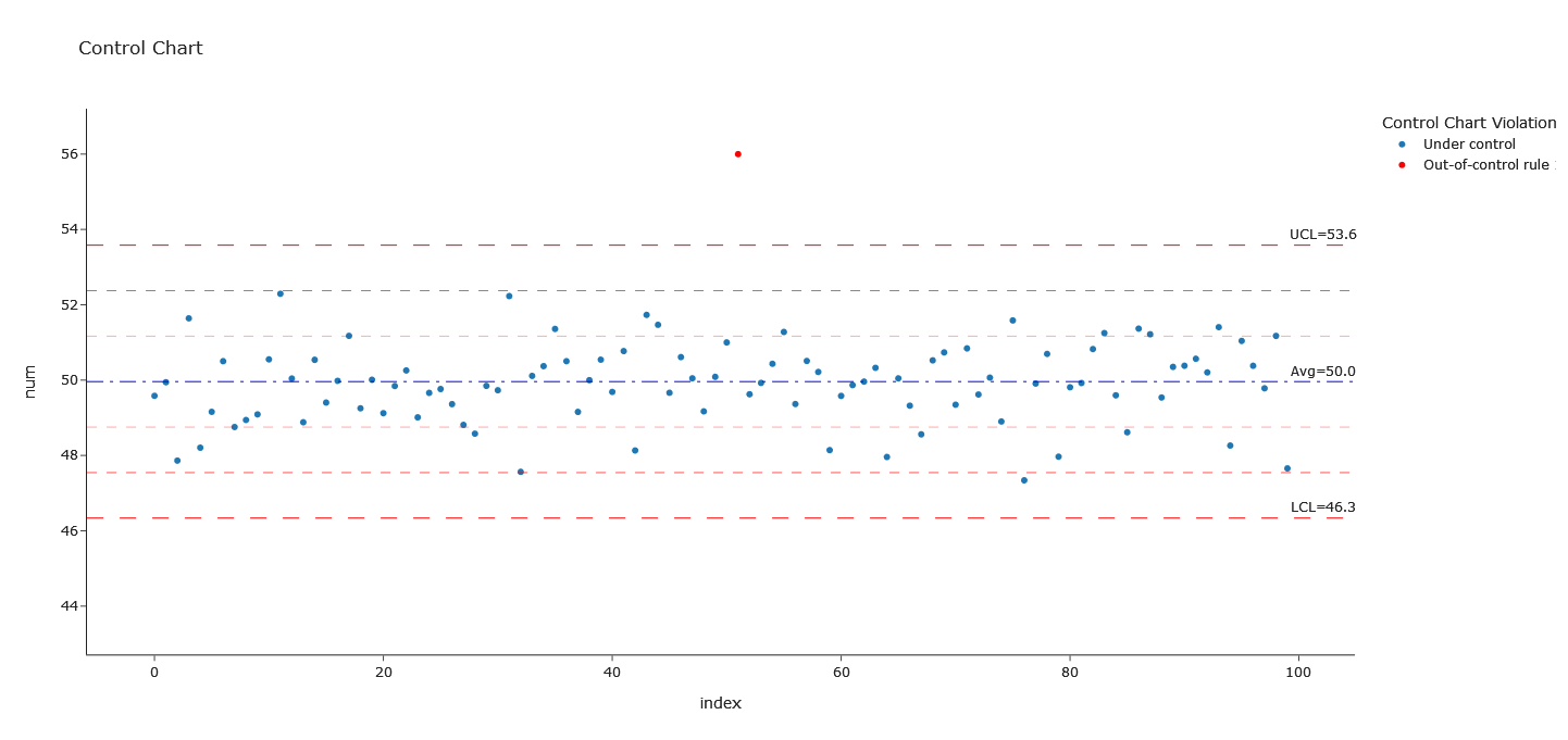
• fccplot: Function to compute and plot a simple (and pretty) Control Chart with Plotly express.

  • Input: Data will be values of the column named variableofinterest and index of the DataFrame as plot index

  • Parameters:

    • path: is provided the graph will be saved in this location.

    • dicorename: allow users to custom names of axis with {“old name” : “desired name”}.

    • forcepower: allow users to force scientific notation 10^n for the y-axis and control limits.

    • addccviol: allow users to add a new column to original data with CC rules check-in.

    • colorby: allow users to color data help to one column values

    • outref: allow users to compute ULC, LCL and mean from given data (pd.Series)

    • hql: allow to plot high quality limit

    • lql: allow to plot low quality limit

    • overinfo: allow to request additional information on ccplot

  • Output: return a DataFrame like data with only Control Chart violations data

• fplotsimple: Plot all columns of a Dataframe as Y and index for x with Plotly express

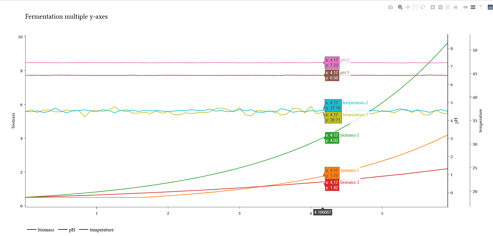
• fplotmultiy: Plot all columns of a Dataframe with autogenerated multi-y-axis and index for x.

  • Input: DataFrame

  • Parameters:

    • path: is provided the graph will be saved in this location

    • yspace: allows users to custom space between yaxis

    • sizep: allows users to custom font size

    • groupby: used character to build group for plotting e.g. groupby=”-” for pH-Biroeactor1 => group pH and subdataset bioreactor1

    • xtitle: allows to custom x title (string is exptected)

  • Output: No output only graph

Usage and code demonstration

• First we create fake datasets: fakedfcc for control chart and fakedfferm for fermentation

  import numpy as np
  import pandas as pd
  import math
  
  # fake process follow-up data
  np.random.seed(2)
  datanorm = np.random.normal(size = 100, loc = 50)
  datanormpower = datanorm*10**5
  datanorm[51] = 56  # add uggly data
  
  fakedfcc = pd.DataFrame(data={"num" : datanorm, "numpower" : datanormpower}, columns=["num", "numpower"])
  
  # fake fermentation data
  time = [time/60 for time in range(0, 60*6, 5)]  # time 5 minutes steps in hours for 6 hours
  pH1 = np.random.normal(size=len(time),loc=6.5,scale=0.005)
  pH2 = np.random.normal(size=len(time),loc=7.2,scale=0.005)
  lagtime = time[20]  # 1.66 h
  biomass1 = [0.5]*20+[0.5*math.exp(0.5*(time-lagtime)) for time in time[20:]]
  biomass2 = [0.5*math.exp(0.5*(time)) for time in time]
  biomass3 = [0.5*math.exp(0.25*(time)) for time in time]
  temp1 = np.random.normal(size=len(time),loc=37,scale=0.5)
  temp2 = np.random.normal(size=len(time),loc=37,scale=0.2)
  
  fakedfferm = pd.DataFrame(data={"pH-1" : pH1,
                                  "pH-2" : pH2,
                                  "biomass-1" : biomass1,
                                  "biomass-2" : biomass2,
                                  "biomass-3" : biomass3,
                                  "temperature-1" : temp1,
                                  "temperature-2" : temp2},
                          columns=["pH-1", "pH-2", "biomass-1", "biomass-2", "biomass-3", "temperature-1", "temperature-2"],
                          index=time)

• What our fake data looks like?

1. fakedfcc

2. fakedfferm

• Demo of fermy

  import fermy
  
  # Control Chart Demo
  fakedfcc.fccplot("num")
  fakedfcc.fccplot("numpower", forcepower=True)
  
  # Fermentation plot Demo
  fakedfferm.fplotmultiy(groupby="-")
  
  # Calculation on fermentation data
  biomassproxy = fakedfferm.iloc[:,2:5]  # selection of biomass related columns
  biomassproxy.fermgrowth()

• Examples of Fermy outputs

• Examples of CINAC like calculations

  import pandas as pd
  import fermy.CINAC
  
  dfcinac = pd.read_csv("https://gitlab.com/Shinuginn/data-sample/-/raw/main/pHkinetic.csv",sep=";",index_col=0)
  desc = dfcinac.cinac()
  print(dfcinac)
  # print dataframe with pH kinetics
  print(desc)
  # print dataframe with cinac descriptors
  # Way to add a new descriptor named newdescr
  def newdescr(seriepH:pd.Series):
      return seriepH.max()
  fermy.CINAC.mycinactable.append(newdescr)
  desc = dfcinac.cinac()
  print(desc)
  # print dataframe with cinac descriptors plus a new one
  # New descriptors can be built bases one of the four mother functions:
  # TimetopH(pHtarget) or pHatTime(Time) or TimeDeltapH (pHini, pHfin, taux:bool) or Ta(timepHini, deltapH)
  # Exemple: slope between pH 5.9 and 5
  def slopebetweenpH5dot9and5(seriepH:pd.Series):
      return fermy.CINAC.TimeDeltapH(seriepH,5.9,5,True)
  fermy.CINAC.mycinactable.append(slopebetweenpH5dot9and5)

• Examples of MTP option

  import fermy.MTP
  
  reads = fermy.MTP.MTPReader("fakepathasstring","fakeMTP")
  print(reads)
  # The MTP reader is set as fakeMTP
  # The path of data file is fakepathasstring
  # Other avaible readers ['Epoch2', 'fakeMTP', 'Tecan96', 'Tecan384', 'Logphase' ,'Fluostar']
  dfMTP = reads.readMTP()
  print(dfMTP)
  # Dataframe with well coordinates as columns and Time of run float of hours as index

Growth Rate Algorithm Description

1. Normalization of data with two user-defined ways. First by divided all data points by a percentage (5 % percent by default) of the maximum value of the distribution. This option may be used if initial data are very noisy (e.g. Biomass proxy coming from a lab scale). Second method divide all data points by the average of the first five points (like in Toussaint et al. 2006). To be more robust regarding next steps each values under 1 is replaced by 1.

2. Then natural logarithm is applied to the normalized data like in Toussaint et al. 2006

3. A smoothing procedure is applied to the corrected biomass proxy by averaging each point with its eight closest neighbors like in Toussaint et al. 2006.

4. The slope of each point was obtained by calculating the slope between the two fourth neighboring points on each side like in Toussaint et al. 2006.

5. The exponential growth rate area (EGRA) is defined where slopes are equal to or greater than 95% of the maximum slope value like in Hall et al 2014.

6. Finally, linear regression is calculated in the EGRA and the slope of the regression gives the maximum (specific) growth rate and the intercept gives Lag time.

Biological signification

• The maximum (specific) growth rate (commonly express in per hours) is the growth rate during logarithmic growth phase (in batch culture) corresponding to the maximum value for the specific condition.

• Lag time (commonly express in hours) is the duration of the phase where growth is absent at the beginning of the culture.

Bibliography

• Hall B.G., Acar H., Nandipati A. and Barlow M. Growth rates made easy. Molecular Biology and Evolution, 31 (1):232-238, 2014.

• Toussaint H., Levasseur G., Gervais-Bird J.,Wellinger R. J., Elela S. A., and Conconi A. A high-throughput method to measure the sensitivity of yeast cells to genotoxic agents in liquid cultures. Mutation Research/Genetic Toxicology and Environmental Mutagenesis, 606 (1-2):92-105, jul 2006.