Physics library to solve pre-universitary physics problems

Project description
easyPhysi
easyPhysi is a physics library to solve pre-university physics problems. The physics areas that are covered by easyPhysi are summarized hereafter. See the main structure to use easyPhysi in Section and also some Examples.
- Kinematics
- Dynamics
- Energy conservation
- Gravitational field
- Electrical field
[!Note] Visit GitHub page at https://github.com/girdeux31/easyPhysi
The main characteristics for easyPhysi are summarized in the following table.
| Characteristic | Value |
|---|---|
| Name | easyPhysi |
| Version | 1.0.1 |
| Author | Carles Mesado |
| Date | 22/12/2023 |
| Size | ~ 40 KiB |
[!NOTE] Notes are use through this document to remark some features.
[!TIP] Tips are use through this document to link relevant examples or show their solution.
0. Index
1. Installation
[!NOTE] easyPhysi is developed and tested with Python 3.10.
Install the package with pip,
pip install easyphysi
or clone the GitHub repository.
gh repo clone girdeux31/easyPhysi
The following third-party modules are requirements.
- matplotlib>=3.7.0
- scipy>=1.11.0
- sympy==1.12
2. Usage
2.0. Main structure
Most pre-university physics problems can be solved following this structure composed of a few lines.
from easyphysi.drivers.universe import Universe
from easyphysi.drivers.body import Body

universe = Universe(dimensions=2)  # 2 o 3 dimensions, default is 2
universe.set('my_prop', value)

body = Body('my_body', dimensions=2)  # 2 o 3 dimensions, default is 2
body.set('my_prop', value)

# define more properties or more bodies as needed

universe.add_body(body)

# add more bodies as needed

solution = universe.physics_equation('my_body').solve('my_unknown')
Let's take the code apart line by line.
- Line 1 and 2: import
UniverseandBodyclasses, these are needed in every single problem solved with easyPhysi. - Line 4: define a universe instance with
Universeclass. Thedimensionsis an optional argument, but only 2 o 3 dimensions are allowed, default is 2. - Line 5: define as many properties for the universe as needed. Universe properties are listed in Table, name and value must be included as arguments. Values must be consistent with property type, see Section.
- Line 7: define as many body instances as needed with
Bodyclass provided that they have different names. Its name must be included as first argument, thedimensionsis an optional argument, but only 2 o 3 dimensions are allowed, default is 2. - Line 8: define as many properties for the body as needed. Body properties are listed in Table, name and value must be included as arguments. Values must be consistent with property type, see Section.
- Line 12: add all defined bodies to the universe (body and universe dimensions must match).
- Line 16: solve the relevant physics equation over a specific body and define the unknown(s). See a list of allowed equations and unknowns in Table.
[!NOTE] Define all bodies and properties before solving any equation.
[!TIP] Example defines a 3D problem.
2.1. Properties
Some properties are defined on a body, while others are defined on a universe. Next Table lists all properties that are allowed to be defined on a body.
[!NOTE] Property names are case sensitive.
| Property | Description | Type | Components |
|---|---|---|---|
| a | Acceleration | Vector | (a_x, a_y[, a_z]) |
| q | Charge | Scalar | q |
| Fe | Electrical force | Vector | (Fe_x, Fe_y[, Fe_z]) |
| Ue | Electrical potential energy | Scalar | Ue |
| Fg | Gravitational force | Vector | (Fg_x, Fg_y[, Fg_z]) |
| Ug | Gravitational potential energy | Scalar | Ug |
| p0 | Initial position | Vector | (p0_x, p0_y[, p0_z]) |
| v0 | Initial velocity | Vector | (v0_x, v0_y[, v0_z]) |
| m | Mass | Scalar | m |
| p | Position | Vector | (p_x, p_y[, p_z]) |
| v | Velocity | Vector | (v_x, v_y[, v_z]) |
Next Table lists all properties that are allowed to be defined in a universe.
| Property | Description | Type | Value |
|---|---|---|---|
| Ee | Electrical field intensity | Vector | (Ee_x, Ee_y[, Ee_z]) |
| Ve | Electrical potential | Scalar | Ve |
| gg | Gravitational field intensity | Vector | (gg_x, gg_y[, gg_z]) |
| Vg | Gravitational potential | Scalar | Vg |
| g | Gravity | Vector | (g_x, g_y[, g_z]) |
| t | Time | Scalar | t |
Use set method in an instanciated body or universe to define its property and define its value according to its type, see Section.
[!NOTE] Units are up to the user. Even though SI is recommended, other systems can be used provided that different units are consistent.
[!NOTE] Force and energy cannot be defined as properties since each force and energy is defined by its own algebraic formula, see Section.
2.1.0. Property types
There are two types of properties: scalars (for example m for mass) and vectors (for example g for gravity).
2.1.0.i Scalars
They are integers of floats, examples follow.
body.set('prop', 250)       # int
body.set('prop', 5.0E-9)    # float
2.1.0.ii Vectors
They are list or tuples (either integers or floats), examples follow.
body.set('prop', [0.0, -9.81])  # list
body.set('prop', (0, +3))       # tuple
The length of value (components) must be the same as defined in the instance of the body or universe the property applies to.
[!NOTE] It is also possible to define only one component in a vector parameter (the other may be irrelevant or unknown). To do so, append
_x,_yor_zto the property name according to the desired axis.
body.set('prop_x', value_x)
body.set('prop_y', value_y)
body.set('prop_z', value_z)
2.1.1. Non-defined properties
Force (mainly used in newton_equation) and energy (mainly used in energy_conservation_equation) cannot be defined as properties in an instanciated body (note that they are not listed in Table). Instead they can be defined in with add_force and add_energy methods over any instanciated body.
body.add_force('my_force', value)
body.add_energy('my_energy', value)
This is designed on purpose because many different forces and energies can apply to a body and could have different algebraic expressions. Thus, the algebraic expression for the force and energy must be defined by the user.
[!TIP] Section shows examples using
newton_equationandadd_forcemethod.
[!TIP] Section shows examples using
energy_conservation_equationandadd_energymethod.
2.2. Special bodies
Special bodies are pre-defined bodies that are ready to be used. There are two types of special bodies: subatomic particles and celestial bodies, see following tables. The mass and charge of subatomic particles are defined in kilograms and coulombs.
| Body | Mass (kg) | Charge (C) |
|---|---|---|
| electron | 9.109e-31 | -1.602e-19 |
| proton | 1.673e-27 | 1.602e-19 |
| neutron | 1.675e-27 | 0.0 |
The mass and position of celestial bodies are defined in kilograms and kilometers.
[!NOTE] The distance of celestial bodies is the average distance to the Sun (except for the Moon, which is the average distance to the Earth) and is defined in the x-axis.
| Body | Mass (kg) | Position (km) |
|---|---|---|
| sun | 1.988e30 | 0.0 |
| mercury | 3.301e23 | 57900000 |
| venus | 4.867e24 | 108200000 |
| earth | 5.972e24 | 149600000 |
| moon | 7.348e22 | 384400 |
| mars | 6.417e23 | 227900000 |
| jupiter | 1.899e27 | 778600000 |
| saturn | 5.685e26 | 1433500000 |
| uranus | 8.682e25 | 2872500000 |
| neptune | 1.024e26 | 4495100000 |
Import them using the following line and use them without instanciating the body or defining its main properties.
from easyphysi.drivers.body import special_body
[!TIP] Example imports an electron from special bodies.
2.3. Equations
The following equations can be solved, each one is a method defined in the Universe class.
[!NOTE] Equation names are case sensitive.
| Equation | Type | Unknowns |
|---|---|---|
| electrical_field_intensity_equation | Vectorial | Ee, p, q |
| electrical_force_equation | Vectorial | Fe, p, q |
| electrical_potential_energy_equation | Scalar | Ue, p, q |
| electrical_potential_equation | Scalar | Ve, p, q |
| energy_conservation_equation | Scalar | - |
| gravitational_field_intensity_equation | Vectorial | gg, m, p |
| gravitational_force_equation | Vectorial | Fg, m, p |
| gravitational_potential_energy_equation | Scalar | Ug, m, p |
| gravitational_potential_equation | Scalar | Vg, m, p |
| linear_position_equation | Vectorial | g, p, p0, t, v0 |
| linear_velocity_equation | Vectorial | g, t, v, v0 |
| newton_equation | Vectorial | a, m |
Use any of these equation in an instance of universe and include the body the equation applies to. Then use the solve method and include the unknown(s) to be solved, see third column in Table.
universe.physics_equation('my_body').solve('my_unknown')
2.3.0. Equation types
There are two types of equations: scalar (for example energy_conservation_equation) and vectorial (for example newton_equation).
2.3.0.i Scalar
Only one unknown is accepted.
out = universe.physics_equation('my_body').solve('my_unk')
[!NOTE] The output is always a list of roots.
2.3.0.ii Vectorial
As many unknowns as universe dimensions are accepted, these must be defined in a list and passed as argument of solve method. Vector components must be append to unknown names, such as a_x, a_y and a_z for acceleration, see Section. The same number of unknowns must be defined as outputs, no name restriction apply for output unknowns.
out_x, out_y = universe.physics_equation('my_body').solve(['unk_x', 'unk_y'])
[!NOTE] The output always has as many list of roots as unknowns.
2.4. Advance features
The most useful features are already defined. However, for the sake of completeness, a few more features for the advance user are defined in this section.
2.4.0. Vector module
Function magnitude is available to obtain a vector module or magnitude.
from easyphysi.utils import magnitude
prop = magnitude((prop_x, prop_y))
[!TIP] Example makes use of
magnitudefunction to calculate the modulo of the velocity.
2.4.1. Define new unknowns
Most unknowns are already defined when a universe or body are instanciated, see Table and Table. However, sometimes new unknowns must be defined, specially with newton_equation and energy_conservation_equation since force and energy algebraic expressions are defined by user, see Section. In these case, Symbol class from Sympy library can be used. Then, the new unknown can be used as argument in solve method to calculate its numerical value.
from sympy import Symbol
my_unknown = Symbol('my_unknown')
[!TIP] Example makes uso of
Symbolclass to define the final velocity (vf) as an unknown and then solve its value.
2.4.2. Substitute variable
Method solve returns numerical values if there is only one unknown (all properties are defined but one), but returns expressions if there is more than one unknown (two or more properties are left undefined). Use subs method to replace an unknown by a specified numerical value.
foo = universe.physics_equation('body').solve('my_unk')  # several undefined properties
out = foo.subs('my_sym', value)
[!Note] There is no need to import
subssince it is a method inherent in any Sympy expression.
[!TIP] Example makes uso of
subsmethod to substitute the friction coefficient by its value.
2.4.3. Get equation from system
In some cases, it is only interesting to solve a specific equation from a vectorial equation (that is a set of equations or a system). The method get_equation can be used over any vectorial equation to return the specific equation, the axis component is expected as method argument.
universe.physics_equation('my_body').get_equation('axis')
[!TIP] Example makes use of
get_equationmethod to extract an equation from a vectorial equation (or set of equations) and, then, solve its unknown.
2.4.4. Solving system of equations
System of equations can be defined -with System class- and solved with solve method. The solve method accepts a list with as many unknowns as equations defined in the system.
from easyphysi.drivers.system import System

equation = universe.physics_equation('body').solve('my_unk')

system = System()
system.add_equation(equation)

# define and add as many equations as needed

x, y, z = system.solve(['x', 'y', 'z'])
[!TIP] Example makes use of
Systemclass to solve a set of equations.
2.4.5. Plotting equations
Method plot can be used over any equation -scalar or vectorial- to plot unknowns in the form of function independent = f(dependent).
universe.physics_equation('my_body').plot(independent, dependent, x_range, points=100, path=None, show=True)
Arguments are described hereafter.
independent: if equation is scalar, then only one independent unknown is expected. If equation is vectorial, then a list with length equal to the number of components (or universe dimensions) is expected.dependent: exactly one unknown is expected.x_range: range to plot for dependent unknown (x-axis).points: number of points to plot, optional argument, default is 100.path: path to save image as file, optional argument, by default it is None and no image is saved.show: ifTruethe plot is shown on screen, optional argument, by default it isTrue.
[!TIP] Example makes uso of
plotmethod to plot a scalar equation (final velocity as a function of initial velocity).
3. Examples
3.0. Kinematics
3.0.0. Example K-0
A ball falls from a roof located 10 m high, forming a 30º angle with the horizontal, with a speed of 2 m/s. Calculate:
a) At what distance from the wall does it hit the ground?
b) The speed it has when it reaches the ground (disregard air friction).
import math

from easyphysi.drivers.body import Body
from easyphysi.drivers.universe import Universe
from easyphysi.utils import magnitude

alpha = math.radians(-30)
g = (0.0, -9.81)
p0 = (0.0, 10.0)
v0 = (2.0*math.cos(alpha), 2.0*math.sin(alpha))
py = 0.0

body = Body('body')  # by default 2D

body.set('p0', p0)
body.set('v0', v0)
body.set('p_y', py)

universe = Universe()  # by default 2D

universe.set('g', g)
universe.add_body(body)

t = universe.linear_position_equation('body').get_equation('y').solve('t')

universe.set('t', t[1])

p_x = universe.linear_position_equation('body').get_equation('x').solve('p_x')

v_x[0], v_y[0] = universe.linear_velocity_equation('body').solve(['v_x', 'v_y'])
v = magnitude((v_x[0], v_y[0]))
[!TIP] Solution:
p_x[0] = 2.30 m, v = 14.15 m/s
3.1. Dynamics
3.1.0. Example D-0
The following ramp has an inclination of 25º. Determine the force that must be exerted on the 250 kg wagon to make it go up with constant velocity:
a) If there is no friction.
b) If 𝜇 = 0.1.
import math
from sympy import Symbol

from easyphysi.drivers.body import Body
from easyphysi.drivers.universe import Universe
from easyphysi.drivers.system import System

mu = Symbol('mu')
alpha = math.radians(25)
m = 250
g = 9.81
W = (-m*g*math.sin(alpha), -m*g*math.cos(alpha))
N = (0.0, m*g*math.sin(alpha))
Fr = (-mu*m*g*math.cos(alpha), 0.0)

body = Body('body')

body.set('m', m)
body.add_force('W', W)
body.add_force('Fr', Fr)
body.add_force('N', N)

universe = Universe()
universe.add_body(body)

a_x[0], a_y[0] = universe.newton_equation('body').solve(['a_x', 'a_y'])
f_00 = m*a_x[0].subs('mu', 0.0)
f_01 = m*a_x[0].subs('mu', 0.1)
[!TIP] Solution:
f_00 = -1036.47 N, f_01 = -1258.74 N
3.1.1. Example D-1
Following previous example, calculate the angle if the acceleration is known.
import math
from sympy import Symbol

from easyphysi.drivers.body import Body
from easyphysi.drivers.universe import Universe
from easyphysi.drivers.system import System

mu = 0.1
sin_alpha = Symbol('sin_alpha')
cos_alpha = Symbol('cos_alpha')
m = 250
g = 9.81
a = (-5.03497308675920, -4.74499424315328)  # from previous example
W = (-m*g*sin_alpha, -m*g*cos_alpha)
N = (0.0, m*g*sin_alpha)
Fr = (-mu*m*g*cos_alpha, 0.0)

body = Body('body')

body.set('m', m)
body.set('a', a)
body.add_force('W', W)
body.add_force('Fr', Fr)
body.add_force('N', N)

universe = Universe()
universe.add_body(body)

sin_alpha, cos_alpha = universe.newton_equation('body').solve(['sin_alpha', 'cos_alpha'])

alpha_from_sin = math.degrees(math.asin(sin_alpha[0]))
alpha_from_cos = math.degrees(math.acos(cos_alpha[0]))
[!TIP] Solution:
alpha_from_sin = 25º, alpha_from_cos = 25º
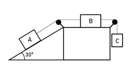
3.1.2. Example D-2
In the system shown in the figure, the three masses are mA = 1 kg, mB = 2 kg, and mC = 1.5 kg. If the coefficient of friction is 𝜇 = 0.223, calculate the acceleration of the system when it is released.
import math
from sympy import Symbol

from easyphysi.drivers.body import Body
from easyphysi.drivers.universe import Universe
from easyphysi.drivers.system import System

g = 9.81
mu = 0.223
alpha = math.radians(30)
ma, mb, mc = 1, 2, 1.5

Fra = (-mu*ma*g*math.cos(alpha), 0.0)
Frb = (-mu*mb*g, 0.0)
Wa = (-ma*g*math.sin(alpha), -ma*g*math.cos(alpha))
Wc = (mc*g, 0.0)

Tab = (Symbol('T2'), 0.0)
Tba = (-Symbol('T2'), 0.0)
Tbc = (Symbol('T1'), 0.0)
Tcb = (-Symbol('T1'), 0.0)

body_a = Body('A')
body_a.set('m', ma)
body_a.add_force('T2', Tab)
body_a.add_force('Fra', Fra)
body_a.add_force('Wa', Wa)

body_b = Body('B')
body_b.set('m', mb)
body_b.add_force('T1', Tbc)
body_b.add_force('T2', Tba)
body_b.add_force('Frb', Frb)

body_c = Body('C')
body_c.set('m', mc)
body_c.add_force('Wc', Wc)
body_c.add_force('T1', Tcb)

universe = Universe()
universe.add_body(body_a)
universe.add_body(body_b)
universe.add_body(body_c)

eq_a = universe.newton_equation('A').get_equation('x')
eq_b = universe.newton_equation('B').get_equation('x')
eq_c = universe.newton_equation('C').get_equation('x')

unknowns = ['T1', 'T2', 'a_x']

system = System()
system.add_equation(eq_a)
system.add_equation(eq_b)
system.add_equation(eq_c)

T1, T2, a_x = system.solve(unknowns)
[!TIP] Solution:
T1[0] = 13.54 N, T2[0] = 7.59 N, a_x[0] = 0.79 m/s2
3.1.3. Example D-3
In the system shown in the figure, the three masses are mA = 1 kg, mB = 2 kg, and mC = 1.5 kg. If the coefficient of friction is 𝜇 = 0.223, calculate the acceleration of the system when it is released.
import math
from sympy import Symbol

from easyphysi.drivers.body import Body
from easyphysi.drivers.universe import Universe
from easyphysi.drivers.system import System
from easyphysi.utils import magnitude

g = 9.81
mu = 0.223
alpha = math.radians(30)
ma = 1
mb = 2
mc = 1.5

Fra = (-mu*ma*g*math.cos(alpha), 0.0)
Frb = (-mu*mb*g, 0.0)
Wa = (-ma*g*math.sin(alpha), -ma*g*math.cos(alpha))
Wc = (mc*g, 0.0)

Tab = (Symbol('T2'), 0.0)
Tba = (-Symbol('T2'), 0.0)
Tbc = (Symbol('T1'), 0.0)
Tcb = (-Symbol('T1'), 0.0)

body = Body('body')
body.set('m', ma+mb+mc)
body.add_force('T2', Tab)
body.add_force('Fra', Fra)
body.add_force('Wa', Wa)
body.add_force('T1', Tbc)
body.add_force('T2', Tba)
body.add_force('Frb', Frb)
body.add_force('Wc', Wc)
body.add_force('T1', Tcb)

universe = Universe()
universe.add_body(body)

a_x, a_y = universe.newton_equation('body').solve(['a_x', 'a_y'])
a = magnitude((a_x[0], a_y[0]))
[!TIP] Solution:
a = 2.05 m/s2
3.2. Energy conservation
3.2.0. Example EC-0
From the top of an inclined plane of 2 m in length and 30º of slope, a 500 g body is allowed to slide with an initial velocity of 1 m/s. Assuming that there is no friction during the journey, with what speed does it reach the base of the plane?
import math
from sympy import Symbol

from easyphysi.drivers.body import Body
from easyphysi.drivers.universe import Universe

m = 1.0
v0 = 1.0
alpha = math.radians(30)
length = 2.0
g = 9.81
h0 = length*math.sin(alpha)
hf = 0.0
vf = Symbol('vf')

Ep0 = m*g*h0
Ek0 = 1/2*m*v0**2
Epf = -m*g*hf
Ekf = -1/2*m*vf**2

body = Body('body')

body.add_energy('Ep0', Ep0)
body.add_energy('Ek0', Ek0)
body.add_energy('Epf', Epf)
body.add_energy('Ekf', Ekf)

universe = Universe()
universe.add_body(body)

vf = universe.energy_conservation_equation('body').solve('vf')
[!TIP] Solution:
vf[0] = 4.54 m/s
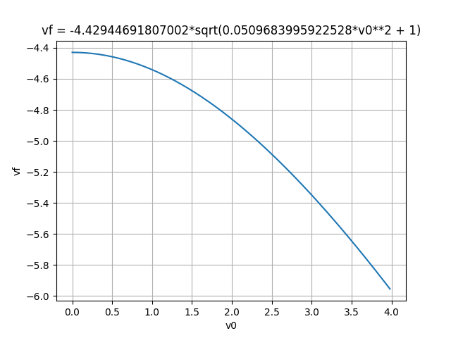
3.2.1. Example EC-1
From the top of an inclined plane of 2 m in length and 30º of slope, a 500 g body is allowed to slide with an initial velocity of 1 m/s. Assuming that there is no friction during the journey, plot the final velocity as a function of the initial velocity.
import math
from sympy import Symbol

from easyphysi.drivers.body import Body
from easyphysi.drivers.universe import Universe

file = 'vf_f_v0.png'

m = 1.0
v0 = Symbol('v0')
alpha = math.radians(30)
length = 2.0
g = 9.81
h0 = length*math.sin(alpha)
hf = 0.0
vf = Symbol('vf')

Ep0 = m*g*h0
Ek0 = 1/2*m*v0**2
Epf = -m*g*hf
Ekf = -1/2*m*vf**2

body = Body('body')

body.add_energy('Ep0', Ep0)
body.add_energy('Ek0', Ek0)
body.add_energy('Epf', Epf)
body.add_energy('Ekf', Ekf)

universe = Universe()
universe.add_body(body)

universe.energy_conservation_equation('body').plot('vf', 'v0', [0, 4], points=200, path=file, show=False)
Solution:
3.2.2. Example EC-2
If upon reaching the flat surface, it collides with a spring of constant k = 200 N/m, what distance will the spring compress?
import math
from sympy import Symbol

from easyphysi.drivers.body import Body
from easyphysi.drivers.universe import Universe

m = 0.5
k = 200.0
v0 = 1.0
alpha = math.radians(30)
length = 2.0
g = 9.81
h0 = length*math.sin(alpha)
hf = 0.0
vf = 0.0
dx = Symbol('dx')

Ep0 = m*g*h0
Ek0 = 1/2*m*v0**2
Epf = -m*g*hf
Ekf = -1/2*m*vf**2
Epe = -1/2*k*dx**2

body = Body('body')

body.add_energy('Ep0', Ep0)
body.add_energy('Ek0', Ek0)
body.add_energy('Epf', Epf)
body.add_energy('Ekf', Ekf)
body.add_energy('Epe', Epe)

universe = Universe()
universe.add_body(body)

dx = universe.energy_conservation_equation('body').solve('dx')
[!TIP] Solution:
dx[0] = 0.227 m
3.2.3. Example EC-3
A 3 kg block situated at a height of 4 m is allowed to slide down a smooth, frictionless curved ramp. When it reaches the ground, it travels 10 m on a rough horizontal surface until it stops. Calculate the coefficient of friction with the horizontal surface.
from sympy import Symbol

from easyphysi.drivers.body import Body
from easyphysi.drivers.universe import Universe

m = 3.0
hc = 0.0
hb = 0.0
vc = 0.0
vb = 8.86
x = 10.0
g = 9.81
mu = Symbol('mu')

Epb = m*g*hb
Ekb = 1/2*m*vb**2
Epc = -m*g*hc
Ekc = -1/2*m*vc**2
Wfr = -mu*m*g*x

body = Body('body')

body.add_energy('Epb', Epb)
body.add_energy('Ekb', Ekb)
body.add_energy('Epa', Epc)
body.add_energy('Eka', Ekc)
body.add_energy('Wfr', Wfr)

universe = Universe()
universe.add_body(body)

mu = universe.energy_conservation_equation('body').solve('mu')
[!TIP] Solution:
mu[0] = 0.40
3.3. Gravitational field
3.3.0. Example GF-0
A point mass A, MA = 3 kg, is located on the xy-plane, at the origin of coordinates. If a point mass B, MB = 5 kg, is placed at point (2, -2) m, determine the force exerted by mass A on mass B.
from easyphysi.drivers.body import Body
from easyphysi.drivers.universe import Universe
from easyphysi.utils import magnitude

body_a = Body('A')
body_a.set('m', 3)
body_a.set('p', (0, 0))

body_b = Body('B')
body_b.set('m', 5)
body_b.set('p', (2, -2))

universe = Universe()
universe.add_body(body_a)
universe.add_body(body_b)

Fg_x, Fg_y = universe.gravitational_force_equation('B').solve(['Fg_x', 'Fg_y'])
Fg = magnitude((Fg_x[0], Fg_y[0]))
[!TIP] Solution:
Fg = 1.25E-10 N
3.3.1. Example GF-1
A point mass A, MA = 3 kg, is located on the xy-plane, at the origin of coordinates. If a point mass B, MB = 5 kg, is placed at point (2, -2) m, determine the work required to move mass B from point (2, -2) m to point (2, 0) m due to the gravitational field created by mass A.
from easyphysi.drivers.body import Body
from easyphysi.drivers.universe import Universe

pa = (0, 0)
pb_0 = (2, -2)
pb_1 = (2, 0)

body_a = Body('A')
body_a.set('m', 3)
body_a.set('p', pa)

body_b = Body('B')
body_b.set('m', 5)

universe = Universe()
universe.add_body(body_a)
universe.add_body(body_b)

body_b.set('p', pb_0)

Ug_0 = universe.gravitational_potential_energy_equation('B').solve('Ug')

body_b.set('p', pb_1)

Ug_1 = universe.gravitational_potential_energy_equation('B').solve('Ug')

W = Ug_0[0] - Ug_1[0]  # W = -AEp = Ug_0 - Ug_1
[!TIP] Solution:
W = 1.47E-10 J
3.3.2. Example GF-2
A point mass m1 = 5 kg is located at the point (4, 3) m. Determine the intensity of the gravitational field created by mass m1 at the origin of coordinates.
from easyphysi.drivers.body import Body
from easyphysi.drivers.universe import Universe
from easyphysi.utils import magnitude

body_a = Body('A')
body_a.set('m', 5)
body_a.set('p', (4, 3))
point = (0, 0)

universe = Universe()
universe.add_body(body_a)

g_x, g_y = universe.gravitational_field_intensity_equation(point).solve(['gg_x', 'gg_y'])
g = magnitude((g_x[0], g_y[0]))
[!TIP] Solution:
g = 1.33E-11 m/s2
3.4. Electrical field
3.4.0. Example EF-0
Problem A3.a 2021 junio coincidentes
At the vertices of a square with a side of 2 m and centered at the origin of coordinates, four electric charges are placed as shown in the figure. Obtain the electric field created by the charges at the center of the square.
from easyphysi.drivers.body import Body
from easyphysi.drivers.universe import Universe
from easyphysi.utils import magnitude

point = (0, 0)

body_1 = Body('1')
body_1.set('q', 5E-9)
body_1.set('p', (-1, +1))

body_2 = Body('2')
body_2.set('q', 5E-9)
body_2.set('p', (+1, +1))

body_3 = Body('3')
body_3.set('q', 3E-9)
body_3.set('p', (+1, -1))

body_4 = Body('4')
body_4.set('q', 3E-9)
body_4.set('p', (-1, -1))

universe = Universe()
universe.add_body(body_1)
universe.add_body(body_2)
universe.add_body(body_3)
universe.add_body(body_4)

Ee_x, Ee_y = universe.electrical_field_intensity_equation(point).solve(['Ee_x', 'Ee_y'])
Ee = magnitude((Ee_x[0], Ee_y[0]))
[!TIP] Solution:
Ee = 12.72 N/C
3.4.1. Example EF-1
Problem A3.b 2021 junio coincidentes
At the vertices of a square with a side of 2 m and centered at the origin of coordinates, four electric charges are placed as shown in the figure. If an electron is launched from the center of the square with a velocity v = 3E4 j m/s, obtain the work done by the electric field when the electron leaves the square through the midpoint of the top side.
from easyphysi.drivers.body import Body, electron
from easyphysi.drivers.universe import Universe

point_0 = (0, 0)
point_1 = (0, 1)

body_1 = Body('1')
body_1.set('q', 5E-9)
body_1.set('p', (-1, +1))

body_2 = Body('2')
body_2.set('q', 5E-9)
body_2.set('p', (+1, +1))

body_3 = Body('3')
body_3.set('q', 3E-9)
body_3.set('p', (+1, -1))

body_4 = Body('4')
body_4.set('q', 3E-9)
body_4.set('p', (-1, -1))

universe = Universe()
universe.add_body(body_1)
universe.add_body(body_2)
universe.add_body(body_3)
universe.add_body(body_4)
universe.add_body(electron)

electron.set('p', point_0)

Ue_0 = universe.electrical_potential_energy_equation('electron').solve('Ue')

electron.set('p', point_1)

Ue_1 = universe.electrical_potential_energy_equation('electron').solve('Ue')

W = Ue_0[0] - Ue_1[0]  # W = -AUe = Ue_0 - Ue_1
[!TIP] Solution:
W = 1.97E-18 J
3.4.2. Example EF-2
A hollow spherical shell with a radius of 3 cm and centered at the origin of coordinates is charged with a uniform surface charge density σ = 2 µC/m2. Obtain the work done by the electric field to move a particle with a charge of 1 nC from the point (0, 2, 0) m to the point (3, 0, 0) m.
from easyphysi.drivers.body import Body
from easyphysi.drivers.universe import Universe

point_0 = (0, 2, 0)
point_1 = (3, 0, 0)

sphere = Body('sphere', dimensions=3)
sphere.set('q', 22.62E-9)
sphere.set('p', (0, 0, 0))

point = Body('point', dimensions=3)
point.set('q', 1E-9)

universe = Universe(dimensions=3)
universe.add_body(sphere)
universe.add_body(point)

point.set('p', point_0)

Ue_0 = universe.electrical_potential_energy_equation('point').solve('Ue')

point.set('p', point_1)

Ue_1 = universe.electrical_potential_energy_equation('point').solve('Ue')

W = Ue_0[0] - Ue_1[0]  # W = -AEp = Ue_0 - Ue_1
[!TIP] Solution:
W = 3.393E-8 J
4. Limitations and bugs
4.0. Limitations
- Trigonometric functions are not able to handle symbols or expressions (for example
math.sin,math.cosormath.atan2). Therefore, position unknown (p) cannot be solved for the following equations (this error is shown:TypeError: Cannot convert expression to float):- electrical_field_intensity_equation
- electrical_force_equation
- gravitational_field_intensity_equation
- gravitational_force_equation
- For the same reason, when defining forces for
newton_equationwithadd_forcemethod, the angle cannot be set as un unknown as it is usually insidemath.sinormath.cosfunctions. Fortunately, since the algebraic formula that defines each force is set by the user, arbitrary unknowns can be set instead ofmath.sin(alpha)ormath.cos(alpha). Then, easily get the angle withmath.asinormath.acos.
[!TIP] Example uses this workaround to solve the unknown angle in a dynamics problem.
4.1. Bugs
Contact the main author if you discover any bug, see Section.
5. Changelog
Main changes:
- 25/06/23 - Initial idea
- 21/12/23 - v1.0.0 first stable version
- 22/12/23 - v1.0.1 minor changes in README and examples
6. License
This project includes GPL-3.0 License. The GPL-3.0 is a free software license that enforces the copyleft principle, requiring any modifications or derivatives to be distributed under the same terms. It mandates source code availability, compatibility with other open-source licenses, and prohibits additional restrictions. The license promotes equal user rights and addresses patent issues.
7. Contact
Feel free to contact mesado31@gmail.com for any suggestion or bug.
Release history Release notifications | RSS feed


Download files
Download the file for your platform. If you're not sure which to choose, learn more about installing packages.
Source Distribution
Built Distribution
Hashes for easyphysi-1.0.1-py3-none-any.whl
| Algorithm | Hash digest | |
|---|---|---|
| SHA256 | e0955c9f868eaafb431104d3421385b21d2fa9fdc38353a3914d1065efd9f5e2 |
|
| MD5 | 73e2fe1be2b6743233cba359002dfe6b |
|
| BLAKE2b-256 | c26e06b170bb9d325eba7b3ea409c73a850b58f3954c8069d1c70c0bf0cd0a7a |


