SZQ lab data analysis core function

Project description
cvmcore


Introduction
The core function of data analysis for plot or data process used by SZQ lab from China Agricultural University
Example usage
from Bio import Phylo
import matplotlib as mpl
import matplotlib.pyplot as plt
from io import StringIO
import matplotlib.collections as mpcollections
from copy import copy

import pandas as pd
import numpy as np
import seaborn as sn

from cvmcore.cvmcore import cvmplot

from scipy.cluster.hierarchy import linkage, dendrogram, complete, to_tree
from scipy.spatial.distance import squareform
mlst = [[np.nan, 19., 12.,  9.,  5.,  9.,  2.],
        [np.nan, 19., 12.,  9.,  5.,  9.,  2.],
        [10., 17., 12.,  9., np.nan,  9.,  2.],
        [10., 19., 12., np.nan,  5.,  9.,  2.],
        [np.nan, 19., 13.,  9.,  5.,  9.,  2.]]
genes = np.char.replace(np.array(np.arange(1, 8), dtype='str'), '', 'gene_', count=1)
samples = np.char.replace(np.array(np.arange(1, 6), dtype='str'), '', 'sample_', count=1)
df_mlst = pd.DataFrame(mlst, index=samples, columns=genes)
diff_matrix = cvmplot.get_diff_df(df_mlst)
diff_matrix
| sample_1 | sample_2 | sample_3 | sample_4 | sample_5 | |
|---|---|---|---|---|---|
| sample_1 | 0 | 0 | 1 | 0 | 1 |
| sample_2 | 0 | 0 | 1 | 0 | 1 |
| sample_3 | 1 | 1 | 0 | 1 | 2 |
| sample_4 | 0 | 0 | 1 | 0 | 1 |
| sample_5 | 1 | 1 | 2 | 1 | 0 |
link_matrix =linkage(squareform(diff_matrix), method='complete')
link_matrix
array([[0., 1., 0., 2.],
       [3., 5., 0., 3.],
       [2., 6., 1., 4.],
       [4., 7., 2., 5.]])
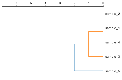
1. Plot a rectangular dendrogram
fig, ax= plt.subplots(1,1)
lableorder, ax = cvmplot.rectree(link_matrix, scale_max=7, labels=samples, ax=ax)
fig.tight_layout()
fig.savefig('screenshots/dendrogram.png')
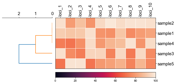
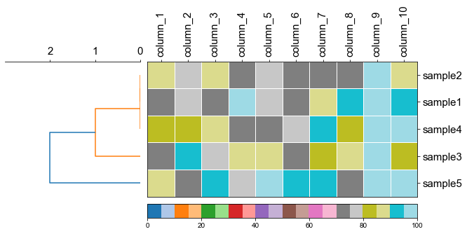
2. Plot rectangular dendrogram with heatmap
#create dataframe
mat = np.random.randint(70, 100, (5, 10))
loci = np.char.replace(np.array(np.arange(1, 11), dtype='str'), '', 'loci_', count=1)
sample = np.char.replace(np.array(np.arange(1, 6), dtype='str'), '', 'sample', count=1)
df_heatmap = pd.DataFrame(mat, index=sample, columns=loci)
#create linkage matrix
diff_matrix = [[0, 0, 1, 0, 1],
               [0, 0, 1, 0, 1],
               [1, 1, 0, 1, 2],
               [0, 0, 1, 0, 1],
               [1, 1, 2, 1, 0]]

linkage_matrix = linkage(squareform(diff_matrix),'complete')
fig, (ax1, ax2) = plt.subplots(1,2,figsize=(8,3), gridspec_kw={'width_ratios': [1, 2]})

fig.tight_layout(w_pad=-2)

row_order, ax1 = cvmplot.rectree(linkage_matrix,labels=sample, no_labels=True, scale_max=3, ax=ax1)
cvmplot.heatmap(df_heatmap, order=row_order, ax=ax2, cbar=True, yticklabel=False)

ax1.set_xticklabels(ax1.get_xticklabels(), fontsize=15)

ax2.set_xticklabels(ax2.get_xticklabels(), rotation=90, fontsize=15)
ax2.set_yticklabels(ax2.get_yticklabels(), fontsize=15)
ax2.xaxis.tick_top()

# fig.tight_layout()
fig.savefig('screenshots/dendrogram_with_heatmap.png', bbox_inches='tight')
[ 5 15 25 35 45]
['sample5', 'sample3', 'sample4', 'sample1', 'sample2']
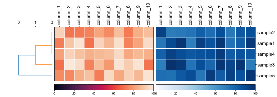
fig, (ax1, ax2, ax3) = plt.subplots(1,3,figsize=(12,3), gridspec_kw={'width_ratios': [1, 2, 2]})

fig.tight_layout(w_pad=-2)

row_order, ax1 = cvmplot.rectree(linkage_matrix,labels=sample, no_labels=True, scale_max=3, ax=ax1)

# remove the yticklabels in ax2
ax2 = cvmplot.heatmap(df_heatmap, order=row_order, ax=ax2, cbar=True, yticklabel=False)
# add ax3 heatmap
ax3 = cvmplot.heatmap(df_heatmap, order=row_order, ax=ax3, cmap='Blues', cbar=True, yticklabel=True)

#set ticklabels property of x or y from ax1, ax2, ax3
ax1.set_xticklabels(ax1.get_xticklabels(), fontsize=15)

ax2.set_xticklabels(ax2.get_xticklabels(), rotation=90, fontsize=15)
ax2.xaxis.tick_top()

ax3.set_xticklabels(ax3.get_xticklabels(), rotation=90, fontsize=15)
ax3.set_yticklabels(ax3.get_yticklabels(), fontsize=15)
ax3.xaxis.tick_top()


# fig.tight_layout()
fig.savefig('screenshots/multiple_heatmap.png', bbox_inches='tight')
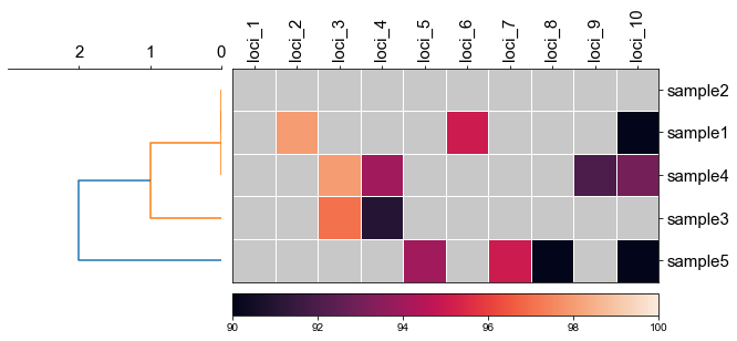
2.1 set minimum value of heatmap
fig, (ax1, ax2) = plt.subplots(1,2,figsize=(8,3), gridspec_kw={'width_ratios': [1, 2]})
fig.tight_layout(w_pad=-2)

order, ax1 = cvmplot.rectree(linkage_matrix,labels=sample, no_labels=True, scale_max=3, ax=ax1)
cvmplot.heatmap(df_heatmap, order=order, ax=ax2, cbar=True, vmin=90)

ax1.set_xticklabels(ax1.get_xticklabels(), fontsize=15)

ax2.set_xticklabels(ax2.get_xticklabels(), rotation=90, fontsize=15)
ax2.set_yticklabels(ax2.get_yticklabels(), fontsize=15)
ax2.xaxis.tick_top()

fig.savefig('screenshots/dendrogram_heatmap_minimumvalue.pdf', bbox_inches='tight')
[ 5 15 25 35 45]
['sample5', 'sample3', 'sample4', 'sample1', 'sample2']
2.2 using cmap to change color
fig, (ax1, ax2) = plt.subplots(1,2,figsize=(8,3), gridspec_kw={'width_ratios': [1, 2]})
fig.tight_layout(w_pad=-2)

order, ax1 = cvmplot.rectree(linkage_matrix,labels=sample, no_labels=True, scale_max=3, ax=ax1)
cvmplot.heatmap(df_heatmap, order=order, ax=ax2, cmap='tab20', cbar=True)

ax1.set_xticklabels(ax1.get_xticklabels(), fontsize=15)

ax2.set_xticklabels(ax2.get_xticklabels(), rotation=90, fontsize=15)
ax2.set_yticklabels(ax2.get_yticklabels(), fontsize=15)
ax2.xaxis.tick_top()
fig.savefig('screenshots/dendrogram_heatmap_cmap.pdf', bbox_inches='tight')
[ 5 15 25 35 45]
['sample5', 'sample3', 'sample4', 'sample1', 'sample2']
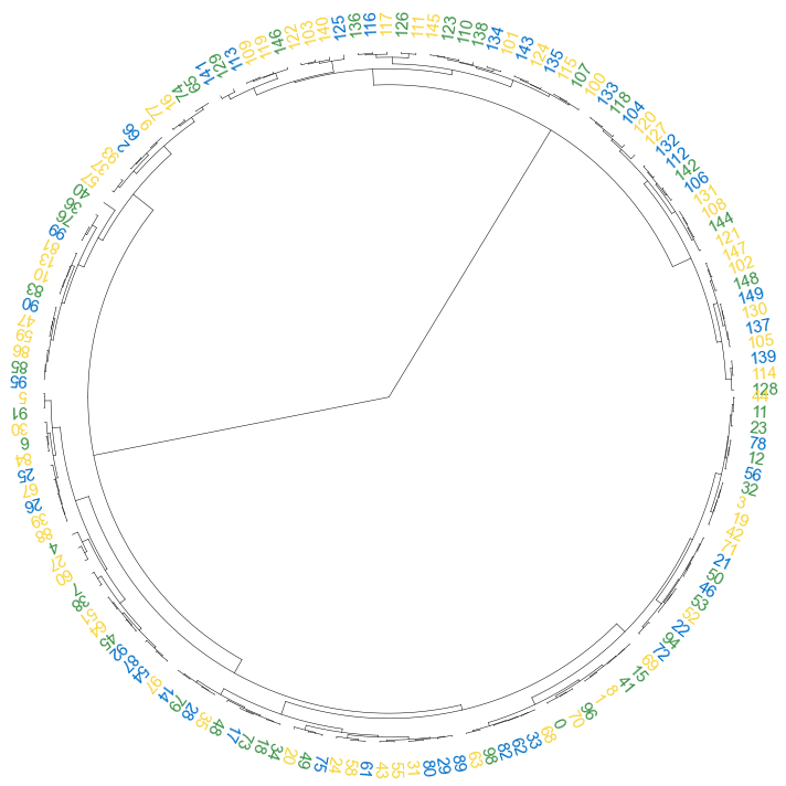
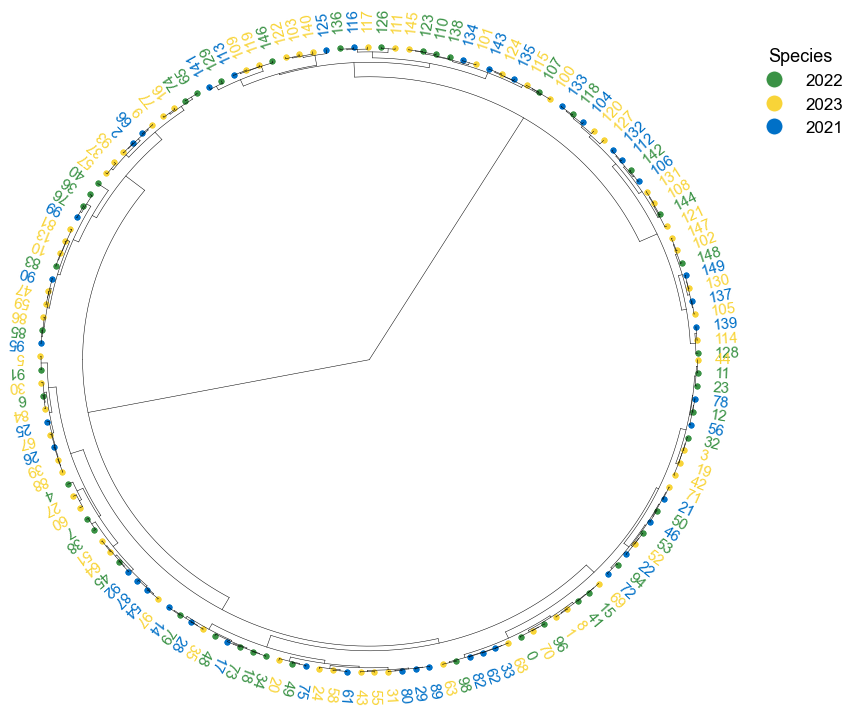
3. Plot a circular dendrogram
# generate two clusters: a with 100 points, b with 50:
np.random.seed(4711)  # for repeatability of this tutorial
a = np.random.multivariate_normal([10, 0], [[3, 1], [1, 4]], size=[100,])
b = np.random.multivariate_normal([0, 20], [[3, 1], [1, 4]], size=[50,])
X = np.concatenate((a, b),)
Z = linkage(X, 'ward')
Z2 = dendrogram(Z, no_plot=True)
# set open angle
fig, ax= plt.subplots(1,1,figsize=(10,10))

cvmplot.circulartree(Z2,addlabels=True, fontsize=10, ax=ax)
fig.tight_layout()
fig.savefig('screenshots/circular_dendrogram.png', bbox_inches='tight')

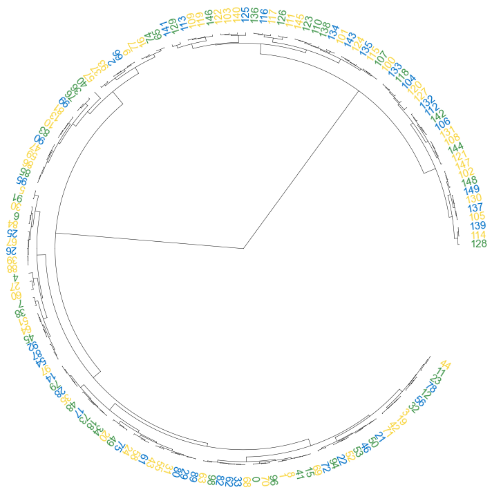
3.1 color label
colors = [{'#0070c7':'2021'}, {'#3a9245':'2022'}, {'#f8d438':'2023'}]
result = np.random.choice(colors, size=150)
label_colors_map = dict(zip(Z2['ivl'], result))
point_colors_map = dict(zip(Z2['ivl'], result))
fig, ax= plt.subplots(1,1,figsize=(10,10))
cvmplot.circulartree(Z2, addlabels=True, branch_color=False, label_colors= label_colors_map, fontsize=15)
fig.tight_layout()
fig.savefig('screenshots/circular_dendrogram_color_label.png')
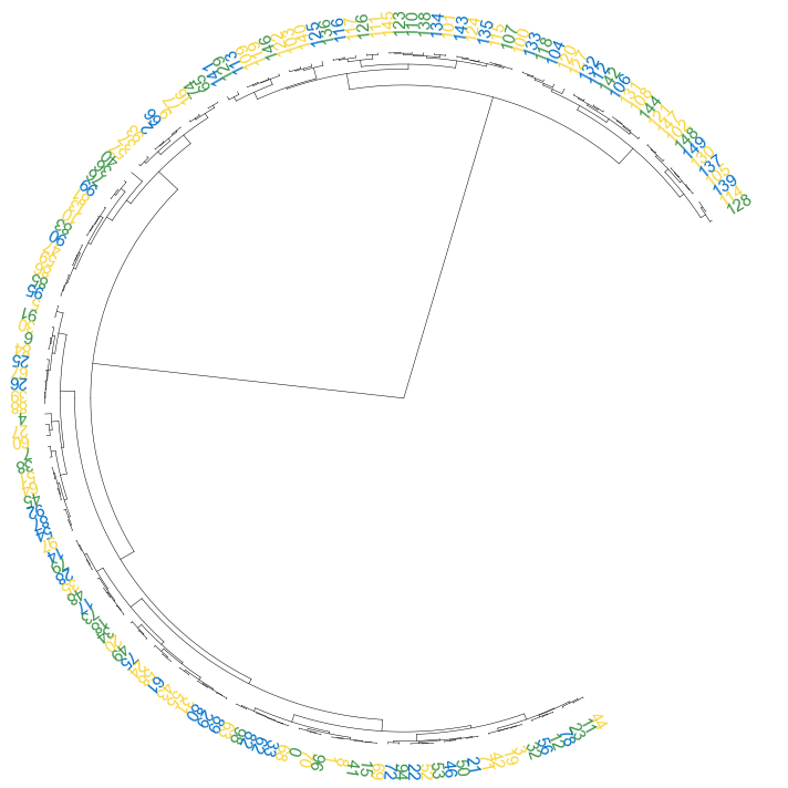
3.2 set open angle
fig, ax= plt.subplots(1,1,figsize=(10,10))
cvmplot.circulartree(Z2, addlabels=True, branch_color=False, label_colors= label_colors_map, fontsize=15, open_angle=30)
fig.tight_layout()
fig.savefig('screenshots/circular_dendrogram_openangle.png')
3.3 set start angle
fig, ax= plt.subplots(1,1,figsize=(10,10))
cvmplot.circulartree(Z2, addlabels=True, branch_color=False, label_colors= label_colors_map, fontsize=15, open_angle=90,
                     start_angle=30
                    )
fig.tight_layout()
fig.savefig('screenshots/circular_dendrogram_startangle.png')
3.4 add point
fig, ax= plt.subplots(1,1,figsize=(12,10))
cvmplot.circulartree(Z2, addlabels=True, branch_color=False, label_colors= label_colors_map, fontsize=15, addpoints=True,
                     point_colors = point_colors_map, point_legend_title='Species', pointsize=25)
fig.tight_layout()
fig.savefig('screenshots/circular_dendrogram_tippoints.png')
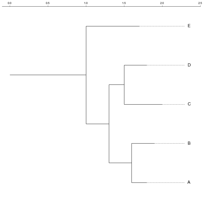
4. Plot phylogenetic tree
tree = "(((A:0.2, B:0.3):0.3,(C:0.5, D:0.3):0.2):0.3, E:0.7):1.0;"
tree = Phylo.read(StringIO(tree), 'newick')
fig, ax= plt.subplots(1,1, figsize=(10, 10))
ax, lable_order = cvmplot.phylotree(tree=tree, color='k', lw=1, ax=ax, show_label=True, align_label=True, labelsize=15)
fig.tight_layout()
fig.savefig('screenshots/phylogenetic tree.png')
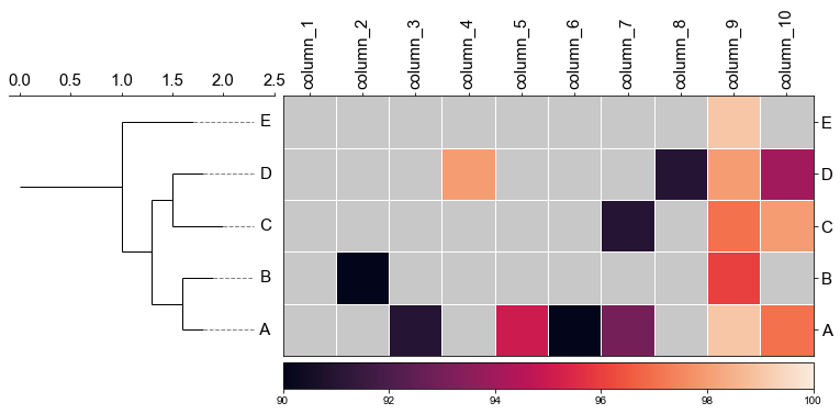
4.1 Plot tree with heatmap
#create dataframe
mat = np.random.randint(70, 100, (5, 10))
col = np.char.replace(np.array(np.arange(1, 11), dtype='str'), '', 'column_', count=1)
strains = ['A', 'B', 'C', 'D', 'E']
df_heatmap = pd.DataFrame(mat, index=strains, columns=col)
df_heatmap
| column_1 | column_2 | column_3 | column_4 | column_5 | column_6 | column_7 | column_8 | column_9 | column_10 | |
|---|---|---|---|---|---|---|---|---|---|---|
| A | 89 | 73 | 91 | 75 | 95 | 90 | 93 | 74 | 99 | 97 |
| B | 73 | 90 | 75 | 89 | 85 | 72 | 82 | 85 | 96 | 82 |
| C | 84 | 82 | 86 | 74 | 72 | 75 | 91 | 83 | 97 | 98 |
| D | 72 | 77 | 72 | 98 | 79 | 73 | 87 | 91 | 98 | 94 |
| E | 88 | 75 | 88 | 73 | 77 | 72 | 74 | 73 | 99 | 86 |
fig,(ax1, ax2)= plt.subplots(1,2, figsize=(8, 3), gridspec_kw={'width_ratios':[1, 2]})
fig.tight_layout(w_pad=-2)
ax1, order = cvmplot.phylotree(tree=tree, color='k', lw=1, ax=ax1, show_label=True, align_label=True, labelsize=15)
cvmplot.heatmap(df_heatmap, order=order, ax=ax2, cbar=True, vmin=90)

ax1.set_xticklabels(ax1.get_xticklabels(), fontsize=15)

ax2.set_xticklabels(ax2.get_xticklabels(), rotation=90, fontsize=15)
ax2.set_yticklabels(ax2.get_yticklabels(), fontsize=15)
ax2.xaxis.tick_top()

fig.savefig('screenshots/phylotree_with_heatmap.pdf')
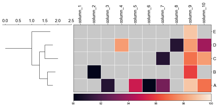
4.2 remove labels at the tip of the tree
fig,(ax1, ax2)= plt.subplots(1,2, figsize=(8, 3), gridspec_kw={'width_ratios':[1, 2]})
fig.tight_layout(w_pad=-2)
ax1, order = cvmplot.phylotree(tree=tree, color='k', lw=1, ax=ax1, show_label=False)
cvmplot.heatmap(df_heatmap, order=order, ax=ax2, cbar=True, vmin=90)

ax1.set_xticklabels(ax1.get_xticklabels(), fontsize=15)

ax2.set_xticklabels(ax2.get_xticklabels(), rotation=90, fontsize=15)
ax2.set_yticklabels(ax2.get_yticklabels(), fontsize=15)
ax2.xaxis.tick_top()

fig.savefig('screenshots/phylotree_with_heatmap-remove_tiplable.pdf', bbox_inches='tight')
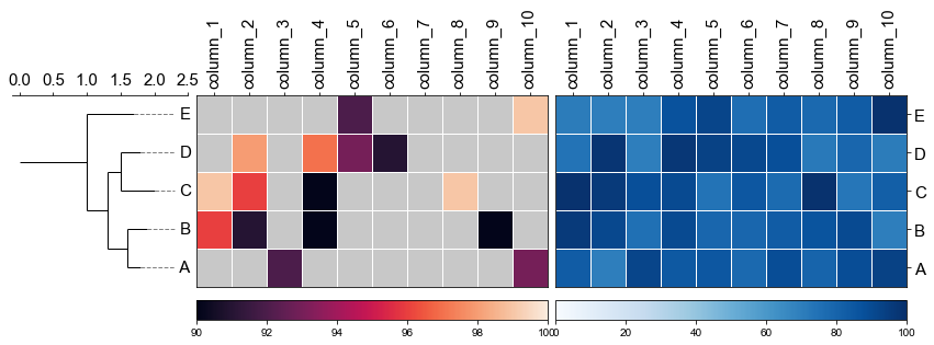
4.3 Plot multiple heatmap with phylotree
fig,(ax1, ax2, ax3)= plt.subplots(1,3, figsize=(12, 3), gridspec_kw={'width_ratios':[1, 2, 2]})
fig.tight_layout(w_pad=-2)
ax1, order = cvmplot.phylotree(tree=tree, color='k', lw=1, ax=ax1, show_label=True, align_label=True, labelsize=15)
ax2 = cvmplot.heatmap(df_heatmap, order=order, ax=ax2, cbar=True, vmin=90, yticklabel=False)
# add ax3 heatmap
ax3 = cvmplot.heatmap(df_heatmap, order=order, ax=ax3, cmap='Blues', cbar=True, yticklabel=True)

#set ticklabels property of x or y from ax1, ax2, ax3
ax1.set_xticklabels(ax1.get_xticklabels(), fontsize=15)

ax2.set_xticklabels(ax2.get_xticklabels(), rotation=90, fontsize=15)
ax2.xaxis.tick_top()

ax3.set_xticklabels(ax3.get_xticklabels(), rotation=90, fontsize=15)
ax3.set_yticklabels(ax3.get_yticklabels(), fontsize=15)
ax3.xaxis.tick_top()


# fig.tight_layout()
fig.savefig('screenshots/phylotree_multiple_heatmap.png', bbox_inches='tight')
5. Gene environment plot
First, you shoud prepare a dataframe from the gff file, The columns should include the feature start, end, strand, label(gene name or whatever you want show next to the arrow) and the arrow color.
| TRACK | START | END | STRAND | LABEL | COLOR |
|---|---|---|---|---|---|
| A | 100 | 900 | -1 | label1 | #ec9631 |
| A | 1100 | 1300 | 1 | label2 | #ec9631 |
| A | 1350 | 1500 | 1 | label3 | #ec9631 |
| A | 1520 | 1700 | 1 | label4 | #ec9631 |
| A | 1900 | 2200 | -1 | label5 | #ec9631 |
| A | 2500 | 2700 | 1 | label6 | #ec9631 |
| A | 2700 | 2800 | -1 | label7 | #ec9631 |
| A | 2850 | 3000 | -1 | label8 | red |
| A | 3100 | 3500 | 1 | label9 | #ec9631 |
| A | 3600 | 3800 | -1 | label10 | #ec9631 |
| A | 3900 | 4200 | -1 | label11 | #ec9631 |
| A | 4300 | 4700 | -1 | label12 | #ec9631 |
| A | 4800 | 4850 | 1 | label13 | #ec9631 |
| B | 100 | 900 | -1 | label14 | #ec9631 |
| B | 1100 | 1300 | 1 | label15 | #ec9631 |
| B | 1350 | 1500 | 1 | label16 | #ec9631 |
| B | 1520 | 1700 | 1 | label17 | #ec9631 |
| B | 1900 | 2200 | -1 | label18 | #ec9631 |
| B | 2500 | 2700 | 1 | label19 | #ec9631 |
| B | 2700 | 2800 | -1 | label20 | #ec9631 |
| B | 2850 | 3000 | -1 | label21 | #ec9631 |
| B | 3100 | 3500 | 1 | label22 | #ec9631 |
| B | 3600 | 3800 | -1 | label23 | #ec9631 |
| B | 3900 | 4200 | -1 | label24 | #ec9631 |
| B | 4300 | 4700 | -1 | label25 | #ec9631 |
| B | 4800 | 4850 | 1 | label26 | #ec9631 |
| C | 100 | 900 | -1 | label27 | #ec9631 |
| C | 1100 | 1300 | 1 | label28 | #ec9631 |
| C | 1350 | 1500 | 1 | label29 | #ec9631 |
| C | 1520 | 1700 | 1 | label30 | #ec9631 |
| C | 1900 | 2200 | -1 | label31 | green |
| C | 2500 | 2700 | 1 | label32 | #ec9631 |
| C | 2700 | 2800 | -1 | label33 | #ec9631 |
| C | 2850 | 3000 | -1 | label34 | #ec9631 |
| C | 3100 | 3500 | 1 | label35 | #ec9631 |
| C | 3600 | 3800 | -1 | label36 | #ec9631 |
| C | 3900 | 4200 | -1 | label37 | #ec9631 |
| C | 4300 | 4700 | -1 | label38 | #ec9631 |
| C | 4800 | 4850 | 1 | label39 | #ec9631 |
| D | 100 | 900 | -1 | label40 | #ec9631 |
| D | 1100 | 1300 | 1 | label41 | #ec9631 |
| D | 1350 | 1500 | 1 | label42 | #ec9631 |
| D | 1520 | 1700 | 1 | label43 | #ec9631 |
| D | 1900 | 2200 | -1 | label44 | #ec9631 |
| D | 2500 | 2700 | 1 | label45 | #ec9631 |
| D | 2700 | 2800 | -1 | label46 | #ec9631 |
| D | 2850 | 3000 | -1 | label47 | #ec9631 |
| D | 3100 | 3500 | 1 | label48 | #ec9631 |
| D | 3600 | 3800 | -1 | label49 | #ec9631 |
| D | 3900 | 4200 | -1 | label50 | #ec9631 |
| D | 4300 | 4700 | -1 | label51 | #ec9631 |
| D | 4800 | 4850 | 1 | label52 | #ec9631 |
| E | 100 | 900 | -1 | label53 | #ec9631 |
| E | 1100 | 1300 | 1 | label54 | #ec9631 |
| E | 1350 | 1500 | 1 | label55 | #ec9631 |
| E | 1520 | 1700 | 1 | label56 | #ec9631 |
| E | 1900 | 2200 | -1 | label57 | #ec9631 |
| E | 2500 | 2700 | 1 | label58 | #ec9631 |
| E | 2700 | 2800 | -1 | label59 | #ec9631 |
| E | 2850 | 3000 | -1 | label60 | #ec9631 |
| E | 3100 | 3500 | 1 | label61 | #ec9631 |
| E | 3600 | 3800 | -1 | label62 | #ec9631 |
| E | 3900 | 4200 | -1 | label63 | #ec9631 |
| E | 4300 | 4700 | -1 | label64 | #ec9631 |
| E | 4800 | 4850 | 1 | label65 | #ec9631 |
5. Plot genes
# Create arrow dictionary
arrow_dict = {k: g.to_dict(orient='records') for k, g in df.set_index('TRACK').groupby(level=0)}

# Define the display order of your tracks
order = ['D', 'A',  'C', 'B', 'E']
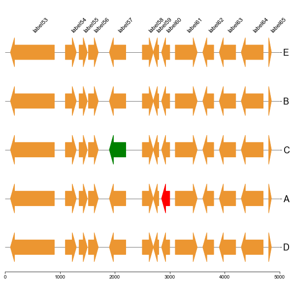
5.1 Plot gene arrows and label on top track
fig, ax = plt.subplots(1,1, figsize=(10,10))
ax = cvmplot.plotgenes(dc=arrow_dict, order=order, ax=ax, max_track_size=5000, addlabels=True, label_track='top')
fig.savefig('screenshots/gene_arrow_top.png', bbox_inches='tight')
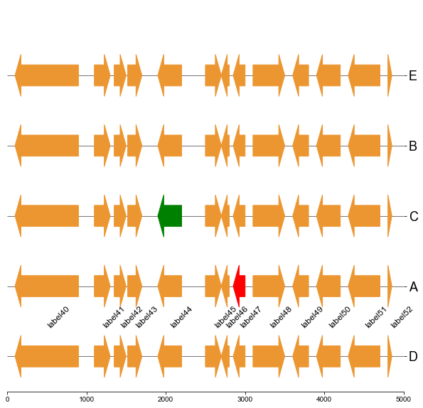
5.2 Plot gene arrows and label on bottom track
fig, ax = plt.subplots(1,1, figsize=(10,10))
ax = cvmplot.plotgenes(dc=arrow_dict, order=order, ax=ax, max_track_size=5000, addlabels=True, label_track='bottom')
fig.savefig('screenshots/gene_arrow_bottom.png', bbox_inches='tight')
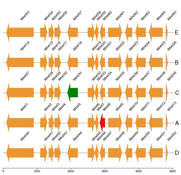
5.3 Plot gene arrows and label on all tracks
fig, ax = plt.subplots(1,1, figsize=(10,10))
ax = cvmplot.plotgenes(dc=arrow_dict, order=order, ax=ax, max_track_size=5000, addlabels=True, label_track='all')
fig.savefig('screenshots/gene_arrow_all.png', bbox_inches='tight')
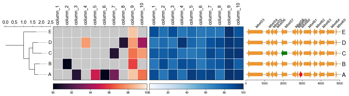
5.4 Plot gene arrows with phylotree and heatmap
Put together!
# Put together
fig,(ax1, ax2, ax3, ax4)= plt.subplots(1,4, figsize=(16, 3), gridspec_kw={'width_ratios':[1, 2, 2, 2]})
fig.tight_layout(w_pad=-2)
ax1, order = cvmplot.phylotree(tree=tree, color='k', lw=1, ax=ax1, show_label=True, align_label=True, labelsize=15)
ax2 = cvmplot.heatmap(df_heatmap, order=order, ax=ax2, cbar=True, vmin=90, yticklabel=False)
# add ax3 heatmap
ax3 = cvmplot.heatmap(df_heatmap, order=order, ax=ax3, cmap='Blues', cbar=True, yticklabel=False)

ax4 = cvmplot.plotgenes(dc=arrow_dict, order=order, ax=ax4, max_track_size=5000, addlabels=True, label_track='top', ylim=(-3, 3))


#set ticklabels property of x or y from ax1, ax2, ax3
ax1.set_xticklabels(ax1.get_xticklabels(), fontsize=15)

ax2.set_xticklabels(ax2.get_xticklabels(), rotation=90, fontsize=15)
ax2.xaxis.tick_top()

ax3.set_xticklabels(ax3.get_xticklabels(), rotation=90, fontsize=15)
ax3.set_yticklabels(ax3.get_yticklabels(), fontsize=15)
ax3.xaxis.tick_top()


# fig.tight_layout()
fig.savefig('screenshots/phylotree_heatmap_withgenes.png', bbox_inches='tight')
Release history Release notifications | RSS feed


Download files
Download the file for your platform. If you're not sure which to choose, learn more about installing packages.
Source Distribution
cvmcore-0.1.2.tar.gz
(756.8 kB
view hashes)
Built Distribution
cvmcore-0.1.2-py3-none-any.whl
(18.1 kB
view hashes)


