Digital Cell Sorter (DCS): a single cell RNA-seq analysis toolkit for clustering, cell type identification, and anomaly detection.
Digital Cell Sorter (DCS): a cell type identification, anomaly detection, and Hopfield landscapes toolkit for single-cell transcriptomics, Sergii Domanskyi, Alex Hakansson, Thomas Bertus, Giovanni Paternostro & Carlo Piermarocchi, PeerJ, 9:e10670 (2021).
The previous publication describing the methodology of cell types identification: Polled Digital Cell Sorter (p-DCS): Automatic identification of hematological cell types from single cell RNA-sequencing clusters, Sergii Domanskyi, Anthony Szedlak, Nathaniel T Hawkins, Jiayin Wang, Giovanni Paternostro & Carlo Piermarocchi, BMC Bioinformatics volume 20, Article number: 369 (2019).
Note: If you want to access the package detailed in our 2019 publication of Polled Digital Cell Sorter go to https://zenodo.org/record/2603265 and download the package (v1.1).
The documentation is available at https://digital-cell-sorter.readthedocs.io/.
These instructions will get you a copy of the project up and running on your machine for data analysis, development or testing purposes.
The software runs in Python >= 3.7
It is highly recommended to install Anaconda. Installers are available at https://www.anaconda.com/distribution/ Whether you already had Anaconda installed or just installed it we recommend to update all packages by running:
conda update conda
With conda, you can create, export, list, remove, and update environments that have different versions of Python and/or packages installed in them. Switching or moving between environments is called activating the environment.
conda create --name DCS
conda activate DCS
Now, in your new environment, the packages can be installed or updated without affecting
your other environments. Note, environments use is not necessary, and the
default (base) is used if you dont set up any other. For more information see
https://docs.conda.io/projects/conda/en/latest/user-guide/tasks/manage-environments.html
Note: use of conda environments (for instance DCS exemplified above) with a high performance computer such as MSU HPCC in a batch job, i.e. not on a development node but submitted to a SLURM queue, requires the following steps. In the slurm script, before line calling your python script, add
conda deactivateto deactivate base environnment andconda activate DCS. After calling the script doconda deactivate. The example testing script is shown below.
SLURM script example:
#!/bin/bash --login
########## Define Resources Needed with SBATCH Lines ##########
#SBATCH --time=00:01:00             # limit of wall clock time - how long the job will run (same as -t)
#SBATCH --ntasks=1                  # number of tasks - how many tasks (nodes) that you require (same as -n)
#SBATCH --cpus-per-task=1           # number of CPUs (or cores) per task (same as -c)
#SBATCH --mem=1G                    # memory required per node - amount of memory (in bytes)
##SBATCH --job-name Name_of_Job     # you can give your job a name for easier identification (same as -J)

########## Command Lines to Run ##########
conda deactivate
conda activate DCS
cd ./                               ### change to the directory where your code is located
python test.py        		    ### call your executable
scontrol show job $SLURM_JOB_ID     ### write job information to output file
conda deactivate
where test.py is the python script where you import and use
DigitalCellSorter.
Install DigitalCellSorter with pip. Most of the dependencies packages
are automatically installed with installation of the latest release
of DigitalCellSorter:
pip install DigitalCellSorter
Alternatively, you can clone and install this module directly from GitHub using:
pip install git+https://github.com/sdomanskyi/DigitalCellSorter
Similarly, one can create a local copy of this project for development purposes, and install the package from the cloned directory:
git clone https://github.com/sdomanskyi/DigitalCellSorter
python setup.py install
Our software uses packages numpy, pandas, matplotlib,
scikit-learn, scipy, mygene, fftw,
fitsne, adjustText and a few other standard Python packages.
Some of the packages used in DigitalCellSorter are not installed by default,
and should by installed by separately if using certain functionality with
Digital Cell Sorter. For example, for network-based clustering
install packages pynndescent, networkx, python-louvain.
Other packages that have to be installed separately are fitsne, umap,
phate and orca. The detailed instructions are below.
With datasets containing less than 2000 cells sklearn.manifold.TSNE is used.
For large datasets Fast Fourier Transform-accelerated Interpolation-based t-SNE (FIt-SNE)
implemented by KlugerLab is used (https://github.com/KlugerLab/FIt-SNE).
To use FIt-SNE the following need to be installed. First update cython by
pip install --upgrade cython
Then install fftw from the conda-forge channel
add conda-forge to your channels, and install fftw:
conda config --add channels conda-forge
conda install fftw
The next installation step is platform specific. To install FI-tSNE for Linux:
pip install fitsne
On macOS Mojave C++ compiler has to be specified explicitly:
env CC=clang CXX=clang++ pip install fitsne
On Windows the FI-tSNE wrapper and executable are already
included with DigitalCellSorter.
To use UMAP layout
pip install umap-learn
To use PHATE
pip install phate
Note, if neither
fitsne,umapnorphateare installedDigitalCellSorterdefaults to PCA two largest principal components for visualization layout.
To use Sankey diagrams that are part of Digital Cell Sorter
install plotly and orca:
conda install -c plotly plotly-orca
conda install -c anaconda psutil
See interactive Hopfield landscape figure and interactive Sankey diagram figure in a browser.
orca is necessary to convert Sankey diagrams to static images.
If for any reason orca is unavailable the Sankey diagrams will be saved as
ineractive HTML figure, that can be opened in a browser (Chrome, Firefox etc.) and
saved as static image. The visualization of DigitalCellSorter are implemented
with matplotlib, allowing all the figures to be saved in either raster or
vactor format. Since plotly can convert simple matplotlib figures
(scatter, line, bar plots, but not heatmaps, splines or other complex patch objects) to
ineractive HTML format DigitalCellSorter can attempt to save any of its figures
as HTML. This is particulatly useful with Projection plots, even though the color
bars are not rendered in HTML figures.
Use the latest release of PyPI package.
For a quick-start demo with a dataset of ~5k PBMCs execute in the terminal and follow prompts:
python -m DigitalCellSorter
The second, more detailed demonstration analysis with step-by-step explanation is discussed here and in the demo section at the end of this README. In your script import the package:
import DigitalCellSorter
Create an instance of class DigitalCellSorter. Here, for simplicity, we use Default parameter values:
DCS = DigitalCellSorter.DigitalCellSorter()
During the initialization a number of parameters can be specified. For detailed list see documentation. Many of these parameters are transfered to DCS attributes thus can be modified after initialization using, e.g.:
DCS.toggleMakeStackedBarplot = False
The input gene expression data is expected in one of the following formats:
- Spreadsheet of comma-separated values
csvcontaining condensed matrix in a form('cell', 'gene', 'expr'). If there are batches in the data the matrix has to be of the form('batch', 'cell', 'gene', 'expr'). Columns order can be arbitrary.
Examples:
| cell | gene | expr |
|---|---|---|
| C1 | G1 | 3 |
| C1 | G2 | 2 |
| C1 | G3 | 1 |
| C2 | G1 | 1 |
| C2 | G4 | 5 |
| ... | ... | ... |
or:
| batch | cell | gene | expr |
|---|---|---|---|
| batch0 | C1 | G1 | 3 |
| batch0 | C1 | G2 | 2 |
| batch0 | C1 | G3 | 1 |
| batch1 | C2 | G1 | 1 |
| batch1 | C2 | G4 | 5 |
| ... | ... | ... | ... |
- Spreadsheet of comma-separated values
csvwhere rows are genes, columns are cells with gene expression counts. If there are batches in the data the spreadsheet the first row should be'batch'and the second'cell'.
Examples:
| cell | C1 | C2 | C3 | C4 |
|---|---|---|---|---|
| G1 | 3 | 1 | 7 | |
| G2 | 2 | 2 | 2 | |
| G3 | 3 | 1 | 5 | |
| G4 | 10 | 5 | 4 | |
| ... | ... | ... | ... | ... |
or:
| batch | batch0 | batch0 | batch1 | batch1 |
|---|---|---|---|---|
| cell | C1 | C2 | C3 | C4 |
| G1 | 3 | 1 | 7 | |
| G2 | 2 | 2 | 2 | |
| G3 | 3 | 1 | 5 | |
| G4 | 10 | 5 | 4 | |
| ... | ... | ... | ... | ... |
Pandas DataFramewhereaxis 0is genes andaxis 1are cells. If the are batched in the data then the index ofaxis 1should have two levels, e.g.('batch', 'cell'), with the first level indicating patient, batch or expreriment where that cell was sequenced, and the second level containing cell barcodes for identification.
Examples:
df = pd.DataFrame(data=[[2,np.nan],[3,8],[3,5],[np.nan,1]],
                  index=['G1','G2','G3','G4'],
                  columns=pd.MultiIndex.from_arrays([['batch0','batch1'],['C1','C2']], names=['batch', 'cell']))
Pandas Serieswhere index should have two levels, e.g.('cell', 'gene'). If there are batched in the data the first level should be indicating patient, batch or expreriment where that cell was sequenced, the second level cell barcodes for identification and the third level gene names.
Examples:
se = pd.Series(data=[1,8,3,5,5],
               index=pd.MultiIndex.from_arrays([['batch0','batch0','batch1','batch1','batch1'],
                                                ['C1','C1','C1','C2','C2'],
                                                ['G1','G2','G3','G1','G4']], names=['batch', 'cell', 'gene']))
Any of the data types outlined above need to be prepared/validated with a function prepare().
Let us demonstrate this on the input of type 1:
df_expr = DCS.prepare('data/testData/dataFileCondensedWithBatches.tsv')
markersDCS.xlsx: An excel book with marker data. Rows are markers and columns are cell types.
'1' means that the gene is a marker for that cell type, '-1' means that this gene is not expressed in this cell type, and '0' otherwise.
This gene marker file included in the package is used by Default.
If you use your own file it has to be prepared in the same format (including the two-line header). Note that only the first worksheet will be read,
and its name can be arbitrary. The first column should contain gene names. The second row should contain cell types, and the first row how
those cell types are grouped. If any of the cell types need to be skipped, have "NA" in the corresponding cell of the first row of that cell type.
Example:
| A | B | C | D | E | F | G | H | I | J | K | L | M | ... |
|---|---|---|---|---|---|---|---|---|---|---|---|---|---|
| B cells | B cells | B cells | T cells | T cells | T cells | T cells | T cells | T cells | T cells | NK cells | NK cells | ... | |
| Marker | B cells naive | B cells memory | Plasma cells | T cells CD8 | T cells CD4 naive | T cells CD4 memory resting | T cells CD4 memory activated | T cells follicular helper | T cells regulatory (Tregs) | T cells gamma delta | NK cells resting | NK cells activated | ... |
| ABCB4 | 1 | 0 | 0 | 0 | 0 | 0 | 0 | 0 | 0 | 0 | 0 | 0 | ... |
| ABCB9 | 0 | 0 | 1 | 0 | 0 | 0 | 0 | 0 | 0 | 0 | 0 | 0 | ... |
| ACAP1 | 0 | 0 | 0 | 0 | 1 | 0 | 0 | 0 | 0 | 0 | 0 | 0 | ... |
| ACHE | 0 | 0 | 0 | 0 | 0 | 0 | 0 | 0 | 0 | 0 | 0 | 0 | ... |
| ACP5 | 0 | 0 | 0 | 0 | 0 | 0 | 0 | 0 | 0 | 0 | 0 | 0 | ... |
| ADAM28 | 1 | 1 | 0 | 0 | 0 | 0 | 0 | 0 | 0 | 0 | 0 | 0 | ... |
| ADAMDEC1 | 0 | 0 | 0 | 0 | 0 | 0 | 0 | 0 | 0 | 0 | 0 | 0 | ... |
| ADAMTS3 | 0 | 0 | 0 | 0 | 0 | 0 | 0 | 0 | 0 | 0 | 0 | 0 | ... |
| ADRB2 | 0 | 0 | 0 | 0 | 0 | 0 | 0 | 0 | 0 | 0 | 0 | 0 | ... |
| AIF1 | 0 | 0 | 0 | 0 | 0 | 0 | 0 | 0 | 0 | 0 | 0 | 0 | ... |
| AIM2 | 0 | 1 | 0 | 0 | 0 | 0 | 0 | 0 | 0 | 0 | 0 | 0 | ... |
| ALOX15 | 0 | 0 | 0 | 0 | 0 | 0 | 0 | 0 | 0 | 0 | 0 | 0 | ... |
| ALOX5 | 0 | 1 | 0 | 0 | 0 | 0 | 0 | 0 | 0 | 0 | 0 | 0 | ... |
| AMPD1 | 0 | 0 | 1 | 0 | 0 | 0 | 0 | 0 | 0 | 0 | 0 | 0 | ... |
| ANGPT4 | 0 | 0 | 1 | 0 | 0 | 0 | 0 | 0 | 0 | 0 | 0 | 0 | ... |
| ... | ... | ... | ... | ... | ... | ... | ... | ... | ... | ... | ... | ... | ... |
Human.MitoCarta2.0.csv: An csv spreadsheet with human mitochondrial genes, created within work
MitoCarta2.0: an updated inventory of mammalian mitochondrial proteins
Sarah E. Calvo, Karl R. Clauser, Vamsi K. Mootha, Nucleic Acids Research, Volume 44, Issue D1, 4 January 2016.
The main class, DigitalCellSorter, includes tools for:
- Pre-preprocessing
- Quality control
- Batch effects correction
- Cells anomaly score evaluation
- Dimensionality reduction
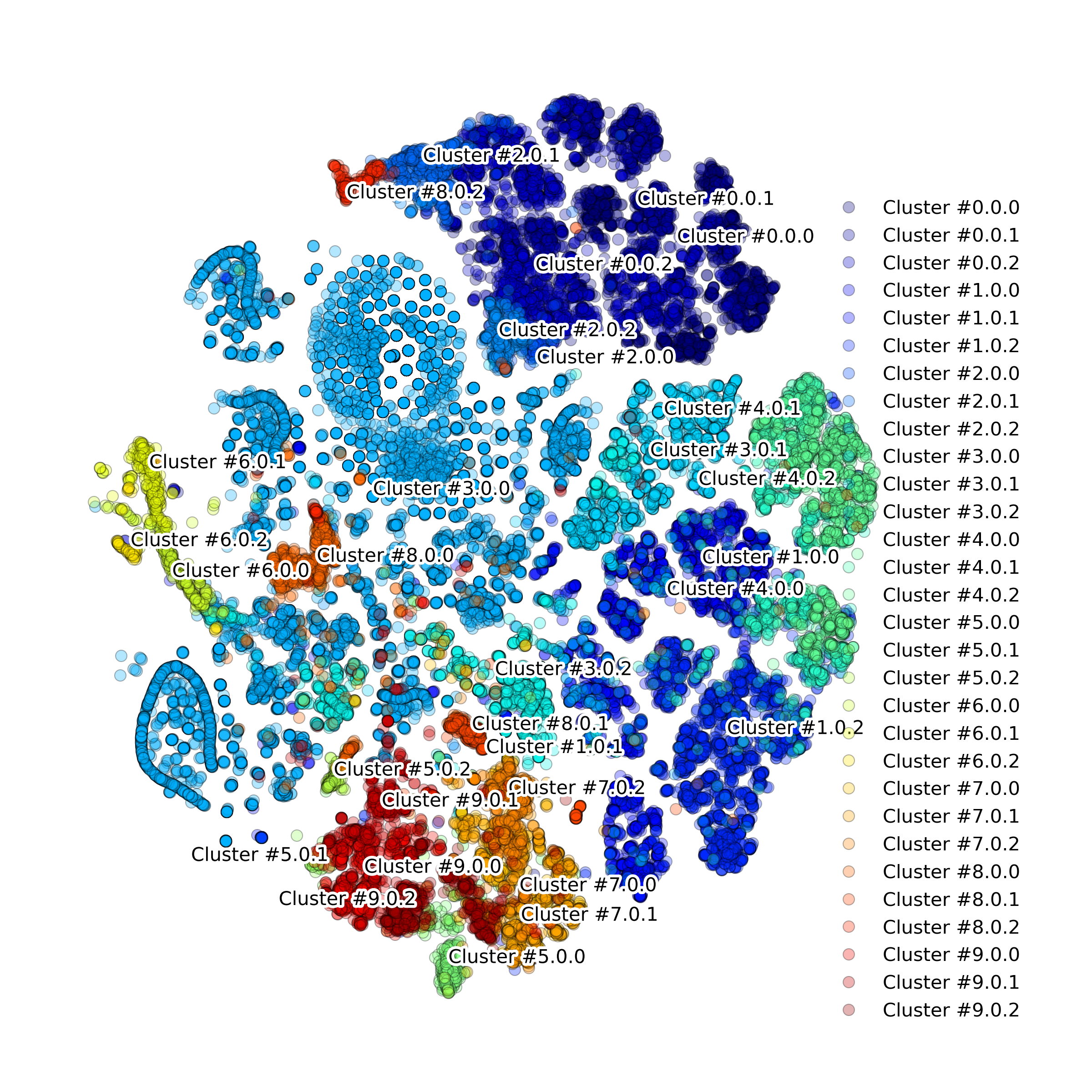
- Clustering
- Annotating cell types
- Vizualization
- Post-processing.
Function visualize() will produce most of the necessary files for post-analysis of the data.
See examples of the visualization tools below.
The visualization tools include:
makeMarkerExpressionPlot(): a heatmap that shows all markers and their expression levels in the clusters, in addition this figure contains relative (%) and absolute (cell counts) cluster sizes

getIndividualGeneExpressionPlot(): 2D layout colored by individual gene's expression
.png?raw=true)
.png?raw=true)
makeVotingResultsMatrixPlot(): z-scores of the voting results for each input cell type and each cluster, in addition this figure contains relative (%) and absolute (cell counts) cluster sizes

makeHistogramNullDistributionPlot(): null distribution for each cluster and each cell type illustrating the "machinery" of the Digital Cell Sorter

makeQualityControlHistogramPlot(): Quality control histogram plots


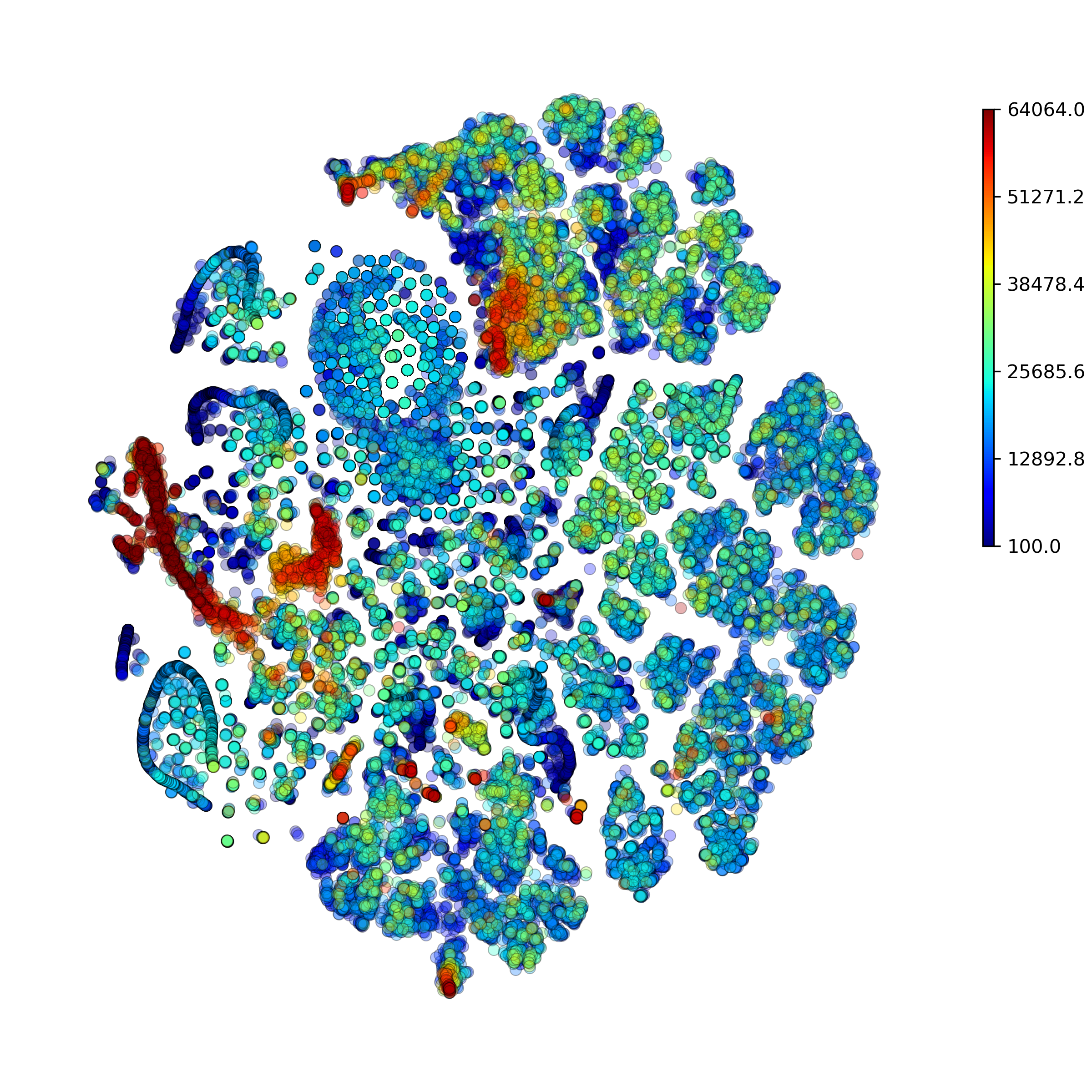
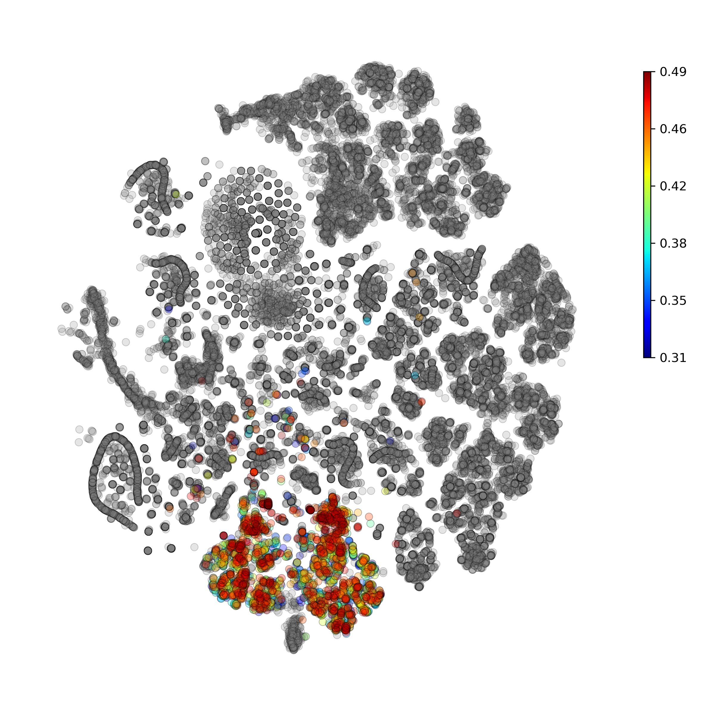
makeProjectionPlot(): 2D layout colored by number of unique genes expressed, number of counts measured, and a faraction of mitochondrial genes..


Effect of batch correction demostrated on combining BM1, BM2, BM3 and processing the data jointly without (left) and with (right) batch correction option:


makeStackedBarplot(): plot with fractions of various cell types


makeSankeyDiagram(): river plot to compare various results

getAnomalyScoresPlot(): plot with anomaly scores per cell

Calculate and plot anomaly scores for an arbitrary cell type or cluster:


getIndividualGeneTtestPlot(): Produce heatmap plot of t-test p-Values calculated gene-pair-wise from the annotated clusters
.png?raw=true)
makePlotOfNewMarkers(): genes significantly expressed in the annotated cell types

We have made an example execution file demo.py that shows how to use DigitalCellSorter.
In the demo, folder data is intentionally left empty.
The data file (cc95ff89-2e68-4a08-a234-480eca21ce79.homo_sapiens.mtx.zip) is about 2.4Gb in size and
will be downloaded with the demo.py script.
Previously the HCA preview data was consolidated in file
ica_bone_marrow_h5.h5and downloadable
from https://preview.data.humancellatlas.org/ (Raw Counts Matrix - Bone Marrow). That file was ~485Mb and containing 378000 cells from 8 bone marrow donors (BM1-BM8).
See details of the script demo.py at:
To execute the complete script demo.py run:
python demo.py
*Note that the HCA BM1 data contains ~50000 sequenced cells, requiring more than 60Gb of RAM (we recommend to use High Performance Computers). If you want to run our example on a regular PC or a laptop, you can use a randomly chosen number of cells:
df_expr.sample(n=5000, axis=1)
All the output files are saved in output directory inside the directory where the demo.py script is.
If you specify any other directory, the results will be generetaed in it.
If you do not provide any directory the results will appear in the root where the script was executed.